How to use Conditional Formatting to format data based on conditions in Excel
How to use Conditional Formatting to format data based on conditions in Excel: Conditional Formatting is a powerful tool that can change the appearance of a cell based on its value, helping viewers quickly identify important data. You can use Conditional Formatting to format data in many ways: change colors, fonts, border styles of one or multiple cells, rows, columns, or entire tables. The format of a cell/column/row changes based on the rules (conditions) you have specified beforehand. This article will guide you on how to use Conditional Formatting to format data based on conditions, emphasizing or distinguishing between data and information stored in Excel.
1. Highlight Cells Rules
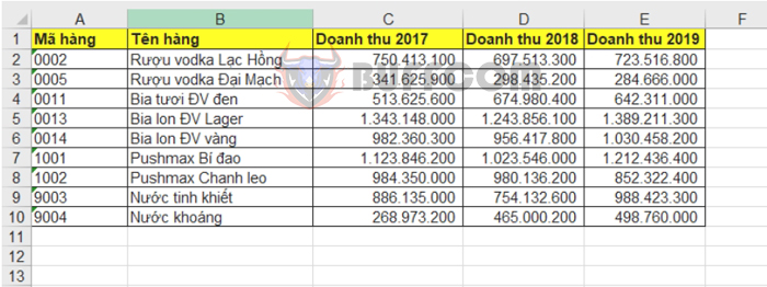
For example, we have a revenue table as follows:
How to use Conditional Formatting to format data based on conditions in Excel
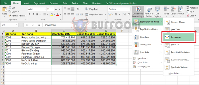
First, you need to select the data range you want to format. Then, select the Home tab => select the Conditional Formatting icon => select Highlight Cells Rules.
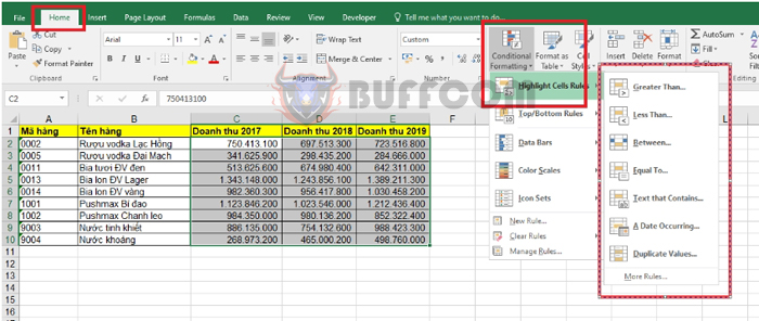 Here you can see the available condition options are:
- Greater than: a value that is greater than a given value.
- Less than: a value that is less than a given value.
- Between: a value that is between a range.
- Equal to: a value that is equal to a given value.
- Text that Contains: a value that contains a certain string of characters.
- A Date Occuring: a value that contains a pre-defined date.
- Duplicate Value: a duplicate value.
For example, if you want to find the revenue values between 500,000,000 and 1,000,000,000, select the Between option.
How to use Conditional Formatting to format data based on conditions in Excel
After the Between window appears, enter 500,000,000 and 1,000,000,000 in the comparison value field. You can choose from pre-defined formats under the Fill option or customize it by selecting Custom Format.
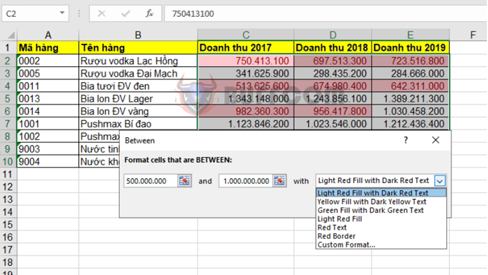 After selecting the options, click OK. The result is that the cells containing values between 500,000,000 and 1,000,000,000 will be highlighted.
2. Top/Bottom Rules
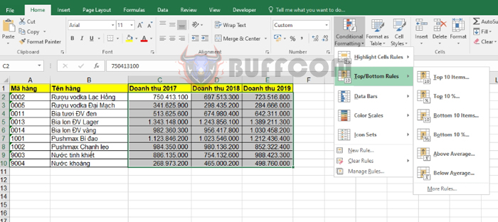
In this section, you have several pre-defined conditions to choose from, such as:
- Top 10 Items: Format the top 10 cells with the highest values.
- Top 10%: Format 10% of cells with the highest values.
- Bottom 10 Items: Format the bottom 10 cells with the lowest values.
- Bottom 10%: Format 10% of cells with the lowest values.
- Above Average: Format cells with values above the average value of the data range.
- Below Average: Format cells with values below the average value of the data range.
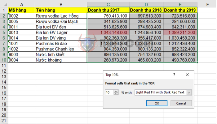
 For example, if you want to format the top 10% cells with the highest values, select the Top 10% option.
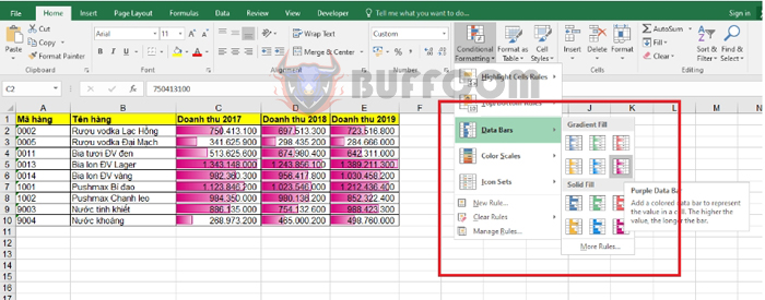
 3. Data Bar
With this format, the size of each cell in the data range will be determined by coloring the cell long or short.
 4. Color Scale
This section will sort the data in ascending or descending order based on the intensity of the color scale.
 These are some common ways to use Conditional Formatting in Excel to format data based on conditions. You can use these techniques to format your data to meet your needs.
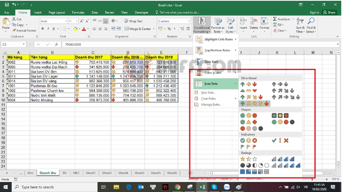
5. Adding icons to value cells (Icon Sets)
With this formatting template, Excel groups data using special icons such as arrows, traffic lights, etc.
How to use Conditional Formatting to format data based on conditions in Excel
Therefore, the above article has guided you on how to use the Conditional Formatting tool to format data based on conditions in Excel. Wishing you success!


