How to use PivotTable to calculate total amount and find duplicate data in Excel
How to use PivotTable to calculate total amount and find duplicate data in Excel: PivotTable is a powerful tool in Excel that can not only analyze data in a spreadsheet, but also be used to calculate total amounts and find and remove duplicate data. In this article, Buffcom.net will share with you the easiest and quickest way to use PivotTable.
1. Creating a PivotTable
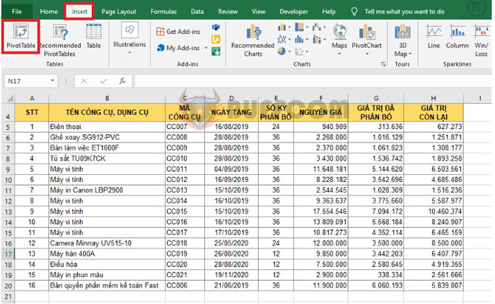
For example, we have a data table as shown below. To create a PivotTable, first, place the cursor in any cell within the data range. Then, select the Insert tab on the toolbar and click on PivotTable in the Tables section.
How to use PivotTable to calculate total amount and find duplicate data in Excel
At this point, the Create PivotTable dialog box will appear. The Table/Range field will display the data range address. Choose where you want the PivotTable report to be placed:
- New Worksheet: place in a new sheet.
- Existing Worksheet: place in the current sheet. If you choose this option, you need to select the location to place the PivotTable in the Location field.
Finally, click OK to create the PivotTable.

How to use PivotTable to calculate total amount and find duplicate data in Excel
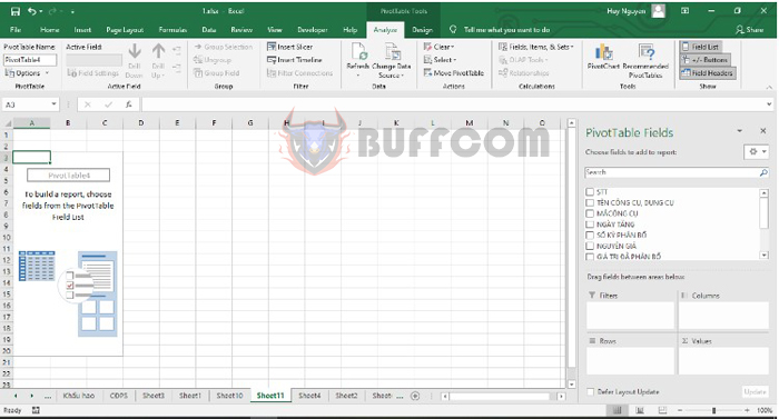
After clicking OK, the PivotTable Fields window will appear on the right side of the screen. This section has two parts:
– Choose fields to add to report: select the data fields to add to the PivotTable report.
– Drag fields between areas below: 4 areas to drop the selected data fields from the Choose fields to add to report section.
- Filter: data filtering area.
- Columns: column names.
- Rows: row names.
- Values: values to display.
How to use PivotTable to calculate total amount and find duplicate data in Excel
2. Finding Duplicate Data
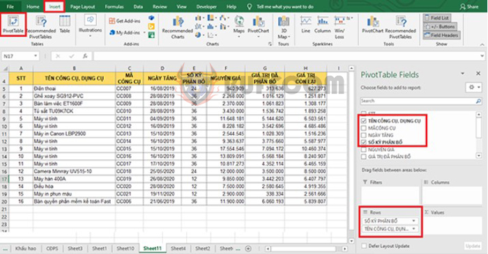
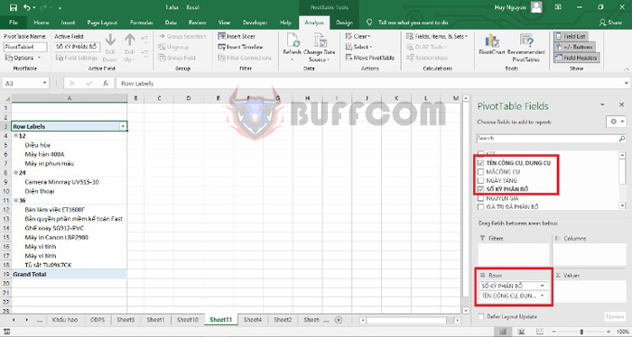
For example, if we need to find tools and equipment in the table with the same depreciation periods, simply check the box next to the Depreciation Period field and the Tool Name or Tool Code field if necessary. The table will automatically filter out tools and equipment with the same depreciation periods. As shown in the picture, there are 3 tools with a 12-month depreciation period, 2 tools with a 24-month depreciation period, and 7 tools with a 36-month depreciation period.
How to use PivotTable to calculate total amount and find duplicate data in Excel
3. Filtering Data
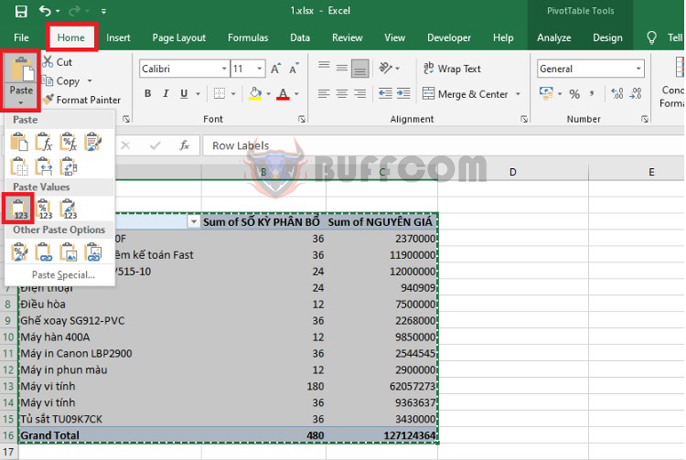
To filter data, first, add the columns you want to display in the table. In this example, I added 3 columns for tool names, depreciation periods, and original values. Next, highlight the entire Pivot table and press Ctrl + C. Then select the Home tab => Paste => Paste Values.
How to use PivotTable to calculate total amount and find duplicate data in Excel
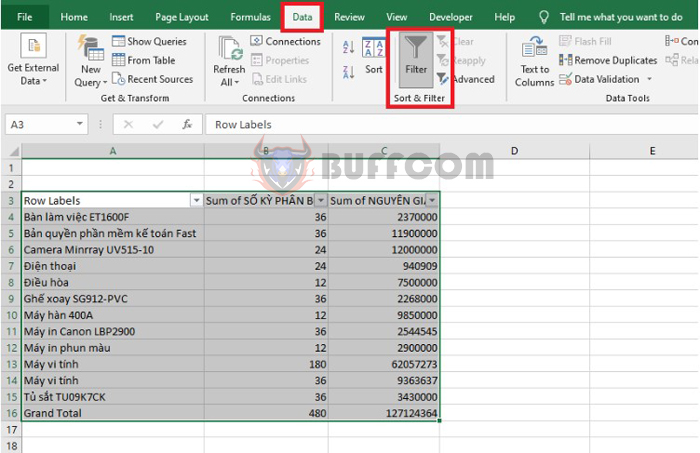
Next, select the Data tab on the toolbar => Filter. The Filter tool will appear in the columns of the table for you to easily filter the data.
How to use PivotTable to calculate total amount and find duplicate data in Excel
In conclusion, PivotTable is a versatile tool in Excel that can be used not only for data analysis but also for calculating totals and finding duplicate data. By following the simple steps outlined in this article, you can quickly and easily use PivotTable to find duplicate data and calculate totals in Excel. Whether you are a beginner or an advanced Excel user, PivotTable can be a useful tool for managing and analyzing your data. With its flexibility and ease of use, PivotTable is a valuable asset in any data analyst’s toolkit.

