How to use the NPV function in Excel to calculate the present value of an investment project

How to use the NPV function in Excel to calculate the present value of an investment project: In this article, Buffcom.net will introduce you to how to use the NPV function in Excel to calculate the present value of an investment project using a discount rate and a series of future cash flows and incomes.
1. NPV function structure
Function syntax: =NPV(rate,value1,[value2],…)
Where:
- Rate: a required argument, is the discount rate.
- Value1, value2, … Value1: required, subsequent values are optional. 1 to 254 arguments representing cash flows and income.
Note:
- Value1, value2 … must have equal time intervals and occur at the end of each period.
- The NPV function uses the order of value1, value2 … to interpret the order of the cash flows.
- Numbers that are blanks, logical values, error values, or text that cannot be converted to numbers will be ignored.
- If the argument is an array or reference, only the numbers in that array or reference are calculated. Blank cells, logical values, text, or error values in the array or reference are ignored.
2. How to use the NPV function
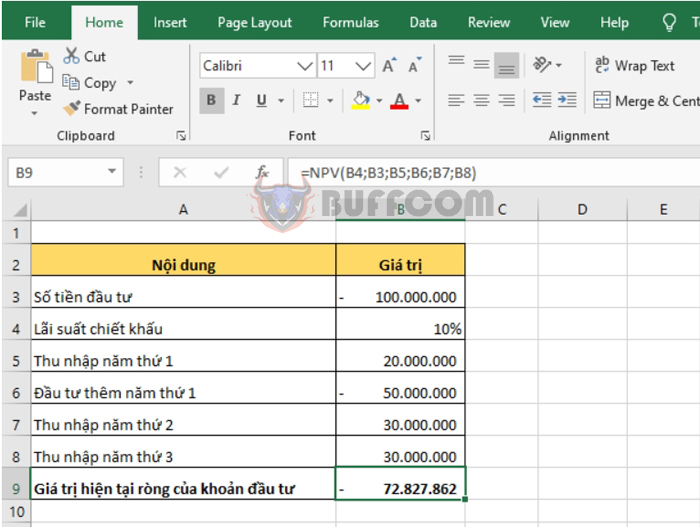
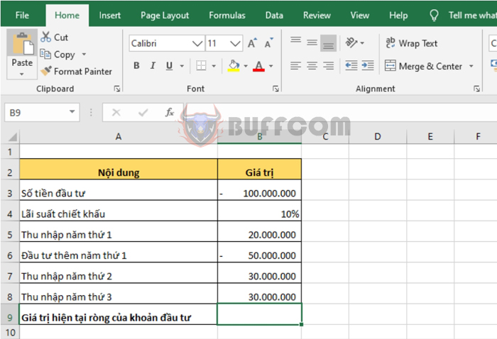
For example, suppose we have an investment project with an initial investment of 100 million. The discount rate is 10% per year. The income in the first year is 20 million. In the second year, an additional 50 million is invested, and the income for the second and third years is 30 million. We need to calculate the present value of this investment project.

How to use the NPV function in Excel to calculate the present value of an investment project
Applying the above function structure, we have the formula to calculate the present value of the investment as follows:
=NPV(B4;B3;B5;B6;B7;B8)
 Thus, this article has guided you on how to use the NPV function to calculate the present value of an investment project. Hopefully, this article will be helpful to you in your work. Wish you success!


