How to Use the TYPE Function in Excel

How to Use the TYPE Function in Excel: The TYPE function in Excel is used to return the data type of a cell. Follow the article below to learn how to use the TYPE function in Excel.

1. Syntax of the TYPE Function

The syntax of the function is: =TYPE(value)

Where:

• Value is a required argument and can be any value such as number, text, or a reference to a cell containing a value.

If the value is a number, the function returns 1. If the value is text, the function returns 2. If the value is a logical value, the function returns 4. If the value is an error value, the function returns 16. If the value is an array, the function returns 64.

Note:

• The TYPE function is most useful when combined with other functions that use different data types, such as the ARGUMENT or INPUT functions.
• The TYPE function cannot be used to determine whether a cell contains a formula or not.

2. How to Use the TYPE Function

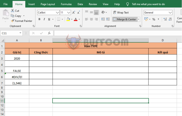
For example, we have values that need to be identified by data type as follows:

• 2020
• FALSE
• #DIV/0!
• {1,546}

Applying the above function syntax, we have the formula to find the data type of cell A3 as follows:

How to Use the TYPE Function in Excel

=TYPE(A3)

Copying the formula for the remaining cells, we will get the following results:

• Cell A3 contains a number, so the function returns 1.
• Cell A4 contains text, so the function returns 2.
• Cell A5 contains a logical value, so the function returns 4.
• Cell A6 contains an error value, so the function returns 16.
• Cell A7 contains an array, so the function returns 64.

How to Use the TYPE Function in Excel

In conclusion, this article has instructed you on how to use the TYPE function in Excel. Good luck!