How to Lookup the Last Value from a Column or a Row in Excel
How to Lookup the Last Value from a Column or a Row in Excel. Excel offers two methods to lookup for the last value from a column or a row. Let’s discuss both formula types and learn when to use them.
Lookup the Last Value (When the Last Value is in the Last Cell)
To use this formula, follow the below steps:
- Enter the INDEX function in a cell.
- Refer to the range of values in the array argument.
- In the rows argument, enter the ROWS function.
- In the ROWS function, refer to the range where you have values.
- Hit enter to get the result.

How to Lookup the Last Value from a Column or a Row in Excel
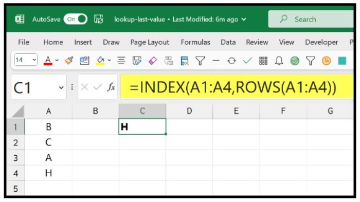
=INDEX(A1:A4,ROWS(A1:A4))
How to Lookup the Last Value from a Column or a Row in Excel
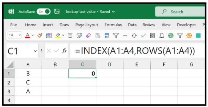
This formula works well when you have a value in the last cell of the range. However, it won’t work when the last cell is empty.
Lookup Last Value in Column
How to Lookup the Last Value from a Column or a Row in Excel
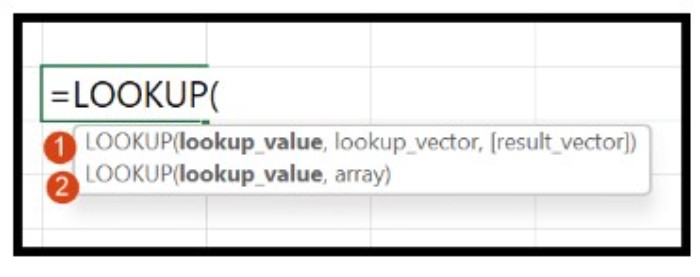
You can use the LOOKUP function to lookup for the last value in a column. The formula will be:
=LOOKUP(2,1/(A:A<>””),A:A)
Here is how this formula works:
How to Lookup the Last Value from a Column or a Row in Excel
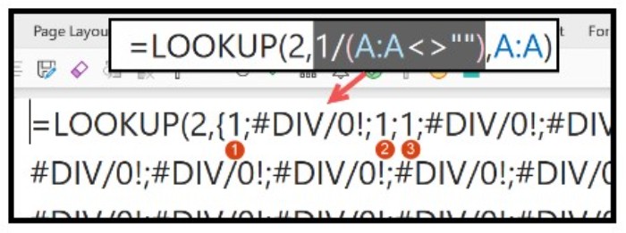
- (A:A<>””) tests whether a cell in column A has a value and returns an array with TRUE or FALSE values.
- 1/(A:A<>””) divides 1 with the above array to get an array of 1s and #DIV/0! errors.
- A:A returns an array with values from column A.

How to Lookup the Last Value from a Column or a Row in Excel
- LOOKUP(2,1/(A:A<>””),A:A) searches for the last 1 in the above array and returns the corresponding value from column A.
Lookup for the Last Value from a Row
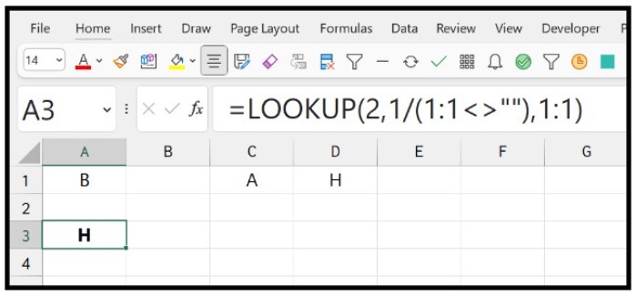
To get the value from the last non-empty cell of a row, change the reference in the above formula.
=LOOKUP(2,1/(1:1<>””),1:1)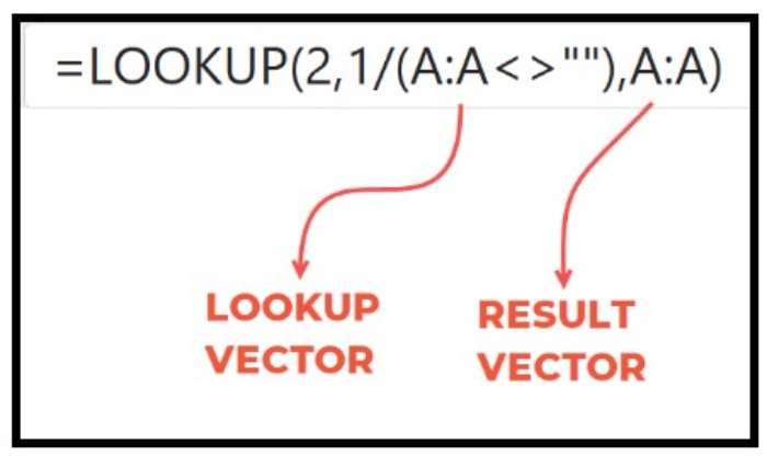
In this formula, we refer to the entire row (Row 1) for the lookup vector and the result vector. 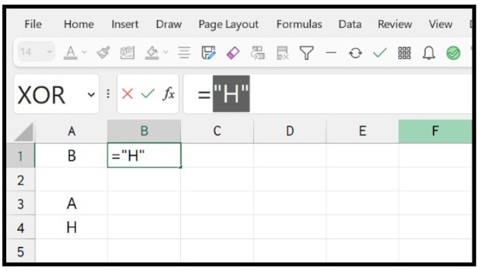 When you hit enter, it returns the value from the last non-empty cell in the row, which is D1 in this case.