Tips for displaying leading zeros in a series of numbers in Excel
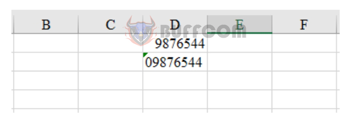
Tips for displaying leading zeros in a series of numbers in Excel: In Excel, when entering a series of numbers that starts with zero, the zero will disappear and only the digits after it will be displayed. This can cause issues when working with data such as phone numbers, postal codes, or employee IDs. To display leading zeros in a series of numbers in Excel, here are two simple methods:
Method 1: Convert the cell to Text format
The first method involves converting the cell (or range of cells) to the Text format. Follow these steps:
Step 1: Select the cell or range of cells that you want to convert to Text format.
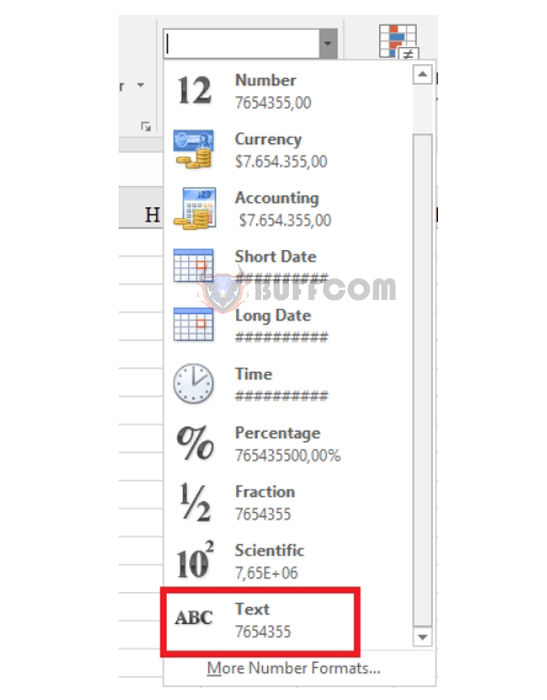
Step 2: On the Home tab, in the Number section, click the drop-down arrow and select Text format.

Tips for displaying leading zeros in a series of numbers in Excel
Select the Text format from the drop-down list.
Tips for displaying leading zeros in a series of numbers in Excel
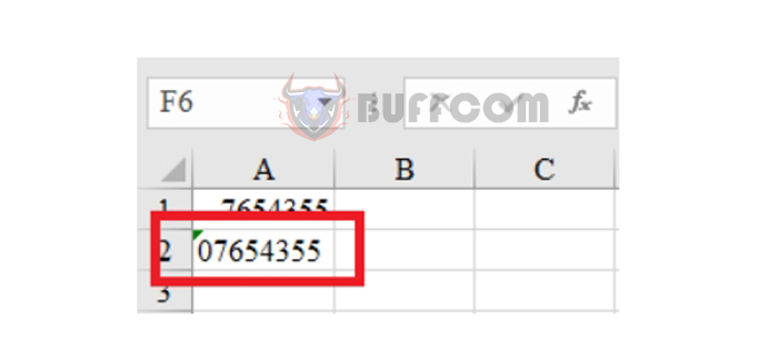
After doing so, you can enter the number as usual, and the leading zero will not be truncated.
However, a green triangle will appear in the upper left corner of the cell. This is an indication that Excel wants to notify you that the data you entered is not text data, but rather numeric data.
Tips for displaying leading zeros in a series of numbers in Excel
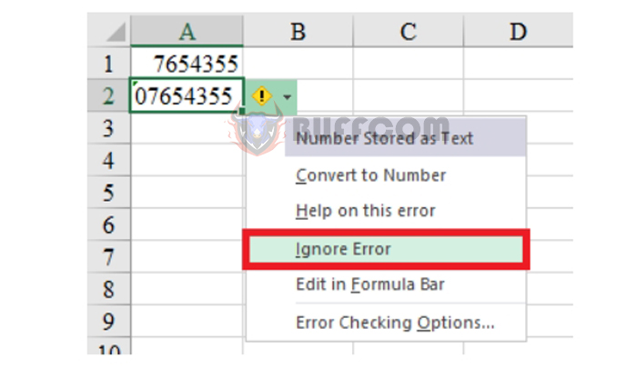
To ignore the error message, click on the yellow error message and select Ignore Error.
Tips for displaying leading zeros in a series of numbers in Excel
Method 2: Use an apostrophe
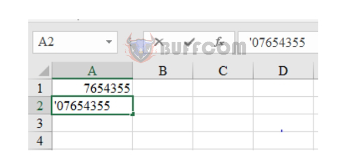
Using an apostrophe (‘) is a manual method for displaying leading zeros in a series of numbers. To do this, simply add an apostrophe before the series of numbers. For example,
Tips for displaying leading zeros in a series of numbers in Excel
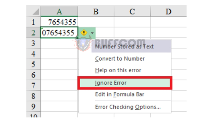
Similar to the first method, a green triangle will appear in the upper left corner of the cell. This is an indication that Excel wants to notify you that the data you entered is not text data, but rather numeric data.
To ignore the error message, click on the yellow error message and select Ignore Error.
Tips for displaying leading zeros in a series of numbers in Excel
Those are two simple methods for displaying leading zeros in a series of numbers in Excel. We hope you find them helpful!


