How to use conditional formatting to highlight due dates in Excel
How to use conditional formatting to highlight due dates in Excel. Missing deadlines can happen, even when we try our best to stay on track. To ensure we don’t overlook important due dates, we can use conditional formatting in Excel to highlight them. This article will guide you through the process.
How to use conditional formatting to highlight due dates in Excel
Highlighting dates matching the current date:
To start, select the data range containing the due dates (e.g., C4:C8).
Go to the Home tab and click on Conditional Formatting in the Styles group.
Choose New Rule from the dropdown menu.
In the dialog box, select “Format Only Cells That Contain” in the upper pane.
From the first dropdown, choose “Dates Occurring.”
In the second dropdown, select “Today.”
Click Format, go to the Font tab, choose the color red, and click OK twice.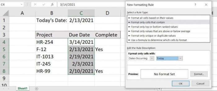
Now, any due date matching the current date will be highlighted in red.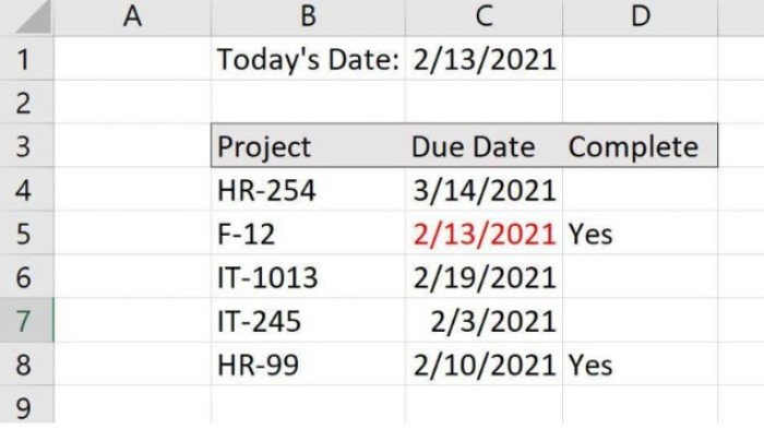
Highlighting the entire row for matching due dates:
If you want to highlight the entire row when the due date matches the current date, follow these steps:
Select the range of data containing the due dates and additional information (e.g., B4:D8).
Go to the Home tab, click on Conditional Formatting, and choose New Rule.
In the dialog box, select “Use a formula to determine which cells to format.”
In the formula field, enter the following function:
=$C4=TODAY()
Click Format, go to the Font tab, choose the color red, and click OK twice.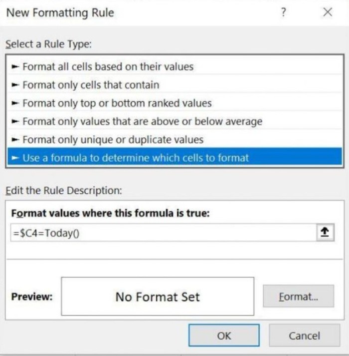
Now, the entire row will be highlighted in red for any task with a due date matching the current date.
Adding a condition to exclude completed tasks:
If you want to further refine the highlighting and exclude completed tasks, follow these steps:
Delete the second rule by selecting “Manage Rules” from the Conditional Formatting dropdown and removing the rule.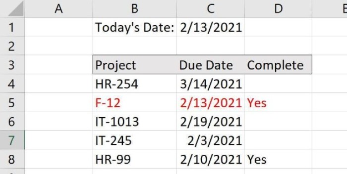
To add the new rule, select the data range (B4:D8).
Go to Conditional Formatting, choose New Rule, and select “Use a formula to determine which cells to format.”
In the formula field, enter the following function:
=AND($C4=TODAY(), $D4<>”Yes”)
Click Format, go to the Font tab, choose the color red, and click OK twice.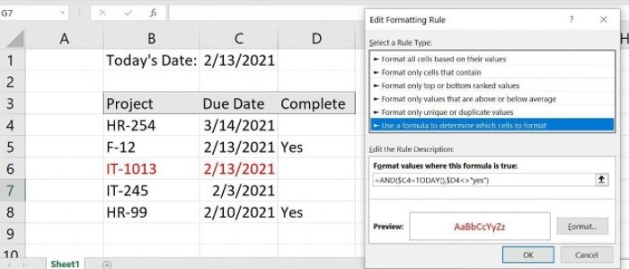
Now, only the rows with due dates matching the current date and incomplete tasks (where column D is not marked as “Yes”) will be highlighted in red.
By using these conditional formatting techniques, you can easily identify due dates that require attention or follow-up. Additionally, you can adapt these methods to create more advanced formatting rules to suit your specific needs.


