Using PivotTable in Excel for reporting and statistics

Latest update as of September 2, 2022: This article provides a detailed guide on how to use PivotTable in Excel. PivotTable is an automatic reporting tool in Excel that helps users perform tasks such as data filtering, report creation, and statistics quickly.

This article will guide you step-by-step on how to use PivotTable in Excel. PivotTable is an Excel tool that helps us analyze data according to a specific requirement. In other words, PivotTable is a tool that allows us to analyze data according to a specific requirement.

Instructions for using PivotTable in Excel

Below is a practical exercise that will help us understand how to use the Pivot function in Excel. You can download the template here to practice creating PivotTable reports.

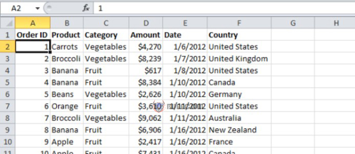The Excel table data represents a detailed sales list of a company selling vegetable products. The details of the order are described as follows: each row represents information on selling a product, for example, Banana, which belongs to a specific commodity, vegetables. There is a certain amount of money sold (amount) for this order and sold on a date (date) in a country.

Practice exercise 1 on how to use PivotTable in Excel will insert a PivotTable into a separate sheet from the available data.

Step 1: Click on the Insert menu and select the PivotTable function.

Step 2: A new window will appear, and you click OK to set up creating a PivotTable in the default mode of Excel.

Explain the Create PivotTable table as follows:

Select A Table or range: the data range needed to create a PivotTable report.

New worksheet: display the PivotTable on a new sheet in the Excel file.

Existing Worksheet: select the display location on the current sheet.

Step 3: The PivotTable appears. First, to calculate the total amount of sales for each product, you follow these steps:

Drag the Product column into the Row Labels area: the list of products will be displayed in rows.

Drag the Amount column into the Values area: the value area to be calculated.

Drag the Country column into the Report area: the value to be filtered.

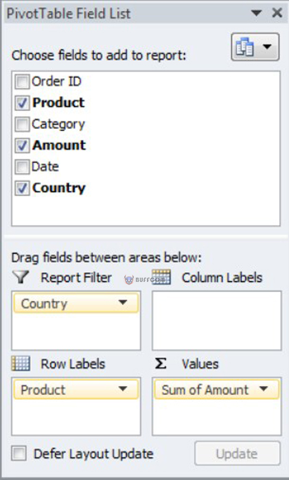And here are the results after completing the above steps.

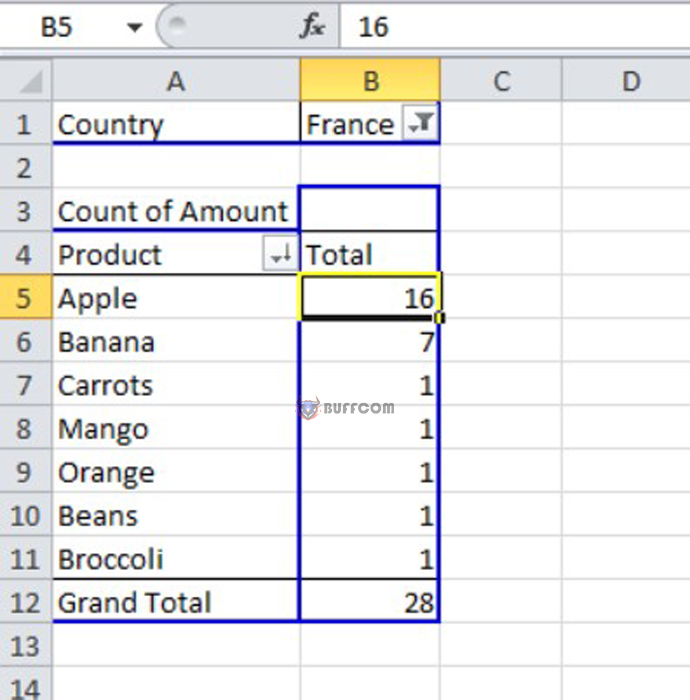
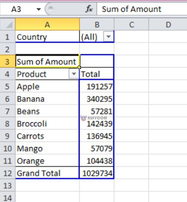In addition to the function of calculating a row’s total by a specific group, such as the result above, calculating the total amount per product, you can customize it to count the number of invoices that contain that product as shown below.

Count the number of invoices containing each product

Right-click on the Sum of Amount being calculated, select Value Field Settings.

Change the calculation method according to the requirement in the Summarize Value by tab.

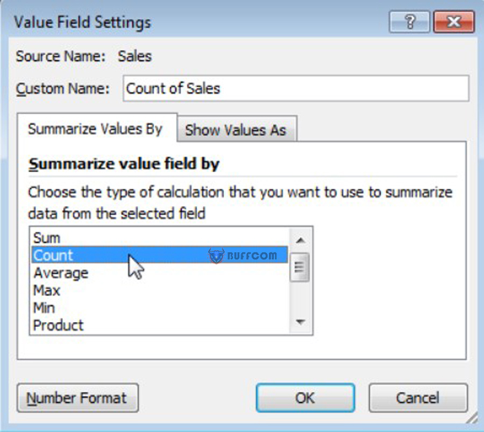Then click OK, and the result will appear below the product list.

I hope this guide helps you understand how to use PivotTable in Excel for reporting and statistics.