3 Reverse Data Tricks in Excel Using Formulas, Easy-to-Understand Illustrated Examples
3 Reverse Data Tricks in Excel Using Formulas. Do you want to reverse data but don’t know how? In this article, I will guide you through 3 very easy and useful tricks that will help you reverse data as desired. Let’s find out together!
Method 1: Reverse Data Tricks in Excel Use SORTBY function to reverse
Syntax: =SORTBY(array, by_array1, [sort_order1], [by_array2, sort_order2],…)
Where:
array: Range or array of cells to be sorted
by_array1: Range or array of cells to sort by
[sort_order1]: The order to sort by. 1 for ascending, -1 for descending. Default is ascending.
[by_array2]: Range or array of cells to sort by
[sort_order2]: The order to sort by. 1 for ascending, -1 for descending. Default is ascending.
Example:
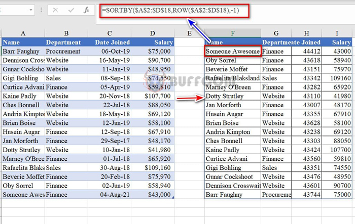
Suppose we have a data table as shown below and to reverse the data using Sortby, you would enter the formula as follows:
=SORTBY($A$2:$D$18,ROW($A$2:$D$18),-1)
3 Reverse Data Tricks in Excel Using Formulas, Easy-to-Understand Illustrated Examples
Method 2: Use POWER QUERY to reverse
Steps:
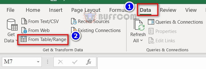
Step 1: Click on any cell within the data range you want to transform, then go to the Data tab –> From table/range.
3 Reverse Data Tricks in Excel Using Formulas, Easy-to-Understand Illustrated Examples
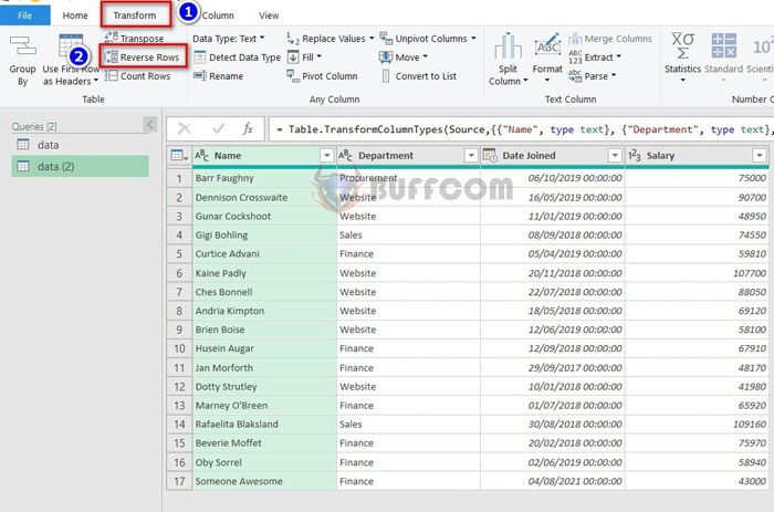
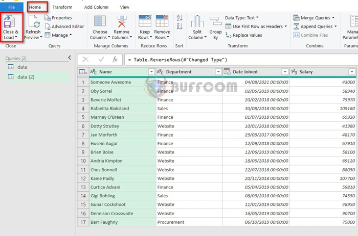
Step 2: The Power Query Editor appears –> select Transpose and click on Reverse Rows. The data range has been reversed.
 Step 3: Go to the Home tab and select Close & load to complete.
3 Reverse Data Tricks in Excel Using Formulas, Easy-to-Understand Illustrated Examples
Method 3: Use formula function to reverse
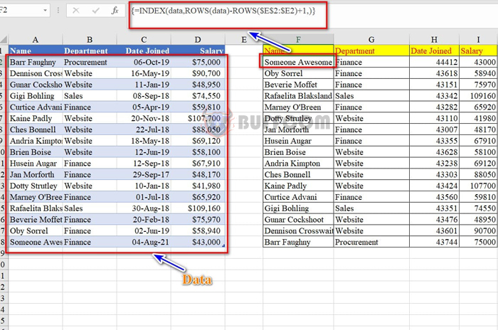
In this case, you would enter the formula as follows:
{=INDEX(data,ROWS(data)-ROWS($E$2:$E2)+1,)}
Where: data is the named data range to be reversed, Index is used to reference the data range, Rows returns the number of rows in the data range.
 So I have shown you how to reverse data in Excel with 3 extremely simple tricks. Good luck with your implementation and don’t forget to rate this article for Buffcom.


