Creating a drop-down list in Excel is simple in 1 minute

Creating a dropdown list in Excel is one of the great ways to impress your boss and colleagues in the workplace. In this article, Buffcom.net will show you 5 simple steps to create a dropdown list in Excel.
Creating a dropdown list in Excel
Microsoft Excel is a powerful spreadsheet software that is widely used for various data-related tasks such as filtering data, sorting data by alphabetical or numerical order, etc. In this article, Buffcom.net will focus on a very useful feature – creating a dropdown list in Excel.
If you are still wondering what a “dropdown list” is, the illustration below will give you an idea of how it works. In this article, Buffcom.net will explain briefly what a dropdown list is and provide a guide on how to create a dropdown list in Excel.
A dropdown list is actually a small window that, when clicked, will drop down a list of different options for you to select quickly.
A dropdown list also provides you with the ability to control exactly what is entered into an Excel cell. This makes the dropdown list a very powerful and popular data validation tool.
Fortunately, creating a dropdown list in Excel is actually very easy if you follow the steps below.
*This tutorial uses Excel 2019/Microsoft 365 (Windows OS). If you use a different version, you can still use the steps below to create a dropdown list in Excel.
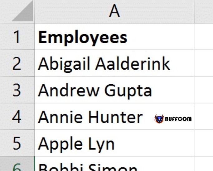
First, we have a sheet with all the names of employees in the company.
This is what we will see when we click on a dropdown list.
 Then, we will have a “small arrow” right next to the cell. When we click on it, it will open a window containing the name data as shown in the image above. You can scroll up and down to browse through the employee name list in the entire sheet, and all of it will be wrapped up in a dropdown list cell.
Now, we will create a dropdown list in cell B1.
Step 1: Click on the “Data” tab.
This step is very easy to perform!
You just need to simply hover your mouse over the “Data” tab and click on it.
 Step 2: Click “Data Validation.”
Click on the “Data validation” button in the middle of the ribbon (don’t click on the small arrow next to the word “Validation” – simply click on the top part of the button as illustrated in the picture) to create a drop-down list in Excel.
 Step 3: Select the “List” option.
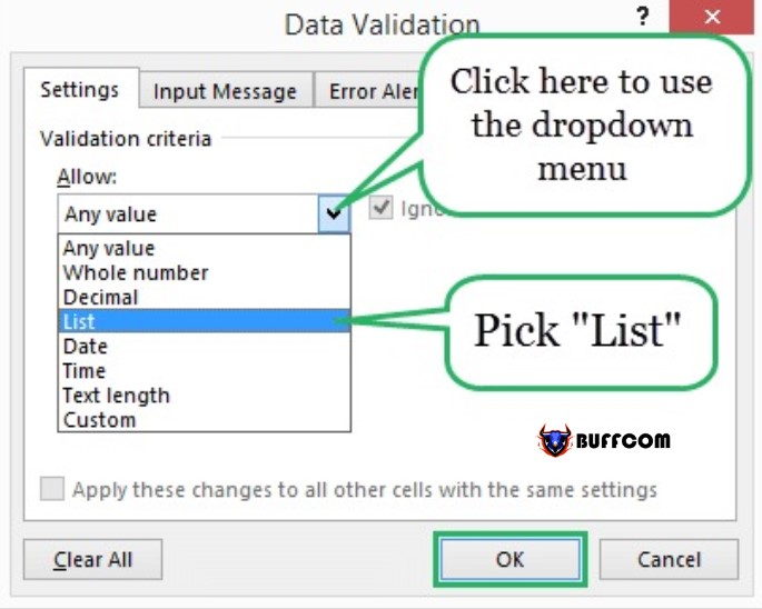
In the dialog box that appears, you need to click on the drop-down list to select the data validation method you want.
Click on the down arrow in the “Allow” field, and in the drop-down list, click on “List”.
 Step 4: Choose the data source to put into the list.
Do you remember the sheet cells containing data that were mentioned at the beginning of the article?
The sheet cells containing the names of all employees in the company will be used as the input data source for the drop-down list.
Now it’s time to declare the data in the range of cells so that Excel can connect the source data (employee names in the sheet) with the drop-down list cell (cell B1).
Click on the “Source:” data field.
Then, click and select all the name data in the sheet.
Click “OK” when done.
 Tip to help you quickly select the entire range of cells without having to drag the mouse like the picture above.
Click on the first data cell (in this case, A2) and then hold down Ctrl + Shift + Down arrow. This will help you quickly select a range of cells in less than a second.
Step 5: The result of the execution!
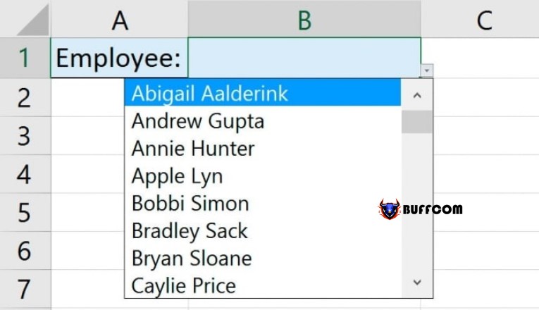 And here is the result of your labor, isn’t it quick and easy?
Above, Buffcom.net has instructed you on how to create a drop-down list in Excel in less than a minute (sometimes less than that). If you are proficient in the above steps, it may only take 10-15 seconds to complete a list like this.
If you find this article useful, please Like & Share to support the team, or leave a comment below to discuss if you have other methods.

