3 Ways to Fill Down Values in Excel

3 Ways to Fill Down Values in Excel. As you have seen, to display data from above into empty cells, we need to use Fill Down. Therefore, Fill Down is used to drag corresponding or similar values down to the appropriate corresponding cells as shown in the image above. Now I will go through 3 ways to Fill Down that I have compiled.
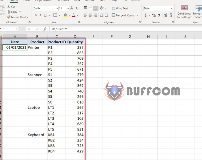 Method 1: Use Goto Special
To use this method, you need to follow these steps:
Step 1: Select the data range, then press the key combination Ctrl + G
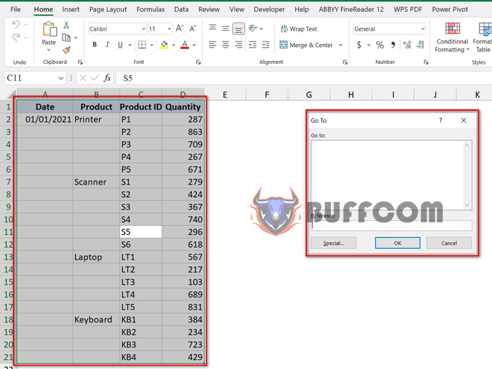 Or you can go to the Home tab, select Find & Select in the Editing group, and choose Go To…
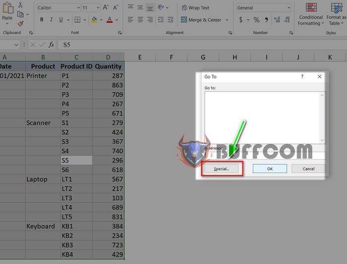
 Step 2: The Go To dialog box appears, here you select Special
 Step 3: Display the Go To Special dialog box, in the dialog box, you select Blank and press Ok.
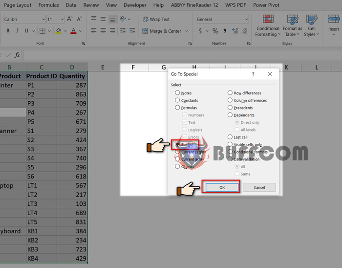 So all the empty cells that need to be filled down have been selected.
Step 4: Then enter the formula: You will press “=”, press the up arrow to get the cell that contains the Fill Down content above.
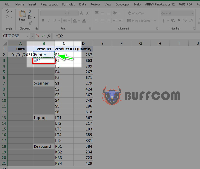 Step 5: Press the key combination Ctrl + Enter to display the value.
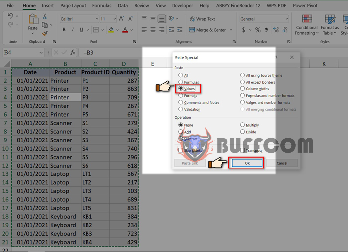
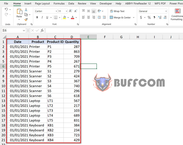 Note: In this case, the cells still have formulas. Therefore, to be able to move data to another position while still keeping the value, you should convert this formula into a value by copying the data range, then right-clicking on the selected data range, choosing Paste => Paste Special, the Paste Special dialog box appears, you select Values and press Ok.
 Method 2: Using VBA in Excel
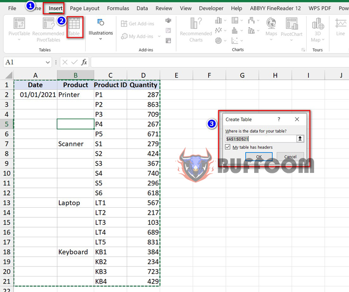
To use this method, your data must be converted to a Table format by: first selecting any cell in the data range, then selecting the Insert tab => Table or pressing Ctrl + T and clicking Ok.
 Steps:
Step 1: Press Alt + F11 to display the VBA interface.
Step 2: Select the sheet containing the data table, right-click and select Insert, then select Module.
 Step 3: Code in the Module window as follows:
Sub FillDown()
Dim xCell As Range
For Each xCell In Selection
If xCell = “” Then
xCell.FillDown
End If
Next
End sub
 Step 4: Then, select the data to be filled down and return to the VBA window. Click Run on the toolbar or press F5 to run the code.
 Step 5: The result will be displayed as shown below.
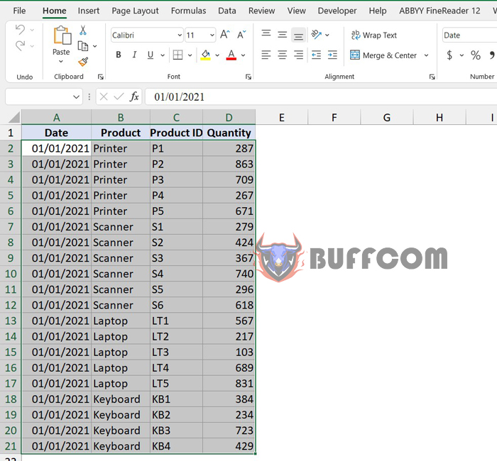 Method 3: Using Power Query
To use this method, your data must be converted to a Table format by: first selecting any cell in the data range, then selecting the Insert tab => Table or pressing Ctrl + T and clicking Ok.
 Steps:
Step 1: Go to the Data tab, select From Table.
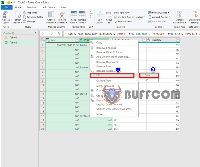
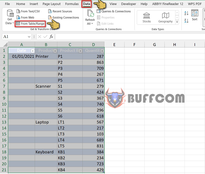 Step 2: The Query Editor window will appear. To select the columns to Fill Down, simply hold down the Ctrl button and select the columns.
Step 3: Right-click on any column name cell, select Fill and select Down.
 Step 4: Once completed, to return to the Excel file, go to the Home tab and select Close & Load.
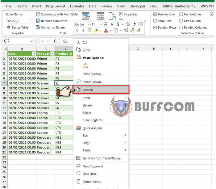
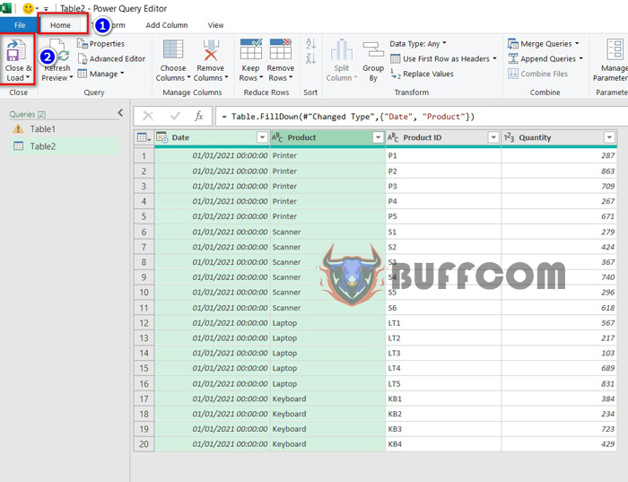 After completion, a new Sheet will be created with the filled-down data. The advantage of this method is that when you change the data in the original table, the changes will be automatically updated by right-clicking and selecting Refresh.
 That’s it, we’ve introduced you to 3 methods for filling down data in Excel. We hope this article is helpful to you. If you found it useful, don’t forget to rate the article below!


