How to Create an Automated Calendar in Excel

How to Create an Automated Calendar in Excel, In today’s society, everyone is overwhelmed with multiple tasks, making it difficult to keep track of personal life. Therefore, a calendar has become an indispensable part of our lives, letting us know the activities we need to do each day. In this article, I will guide you on how to create a calendar for the days of the month and 12 months of the year, where you can change the month and year to keep track of your schedule.

Create a dropdown list of the month and year

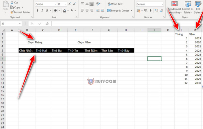
First, enter the days from Sunday to Monday. Highlight from Monday to Sunday and adjust the font size and color accordingly. For example, from Sunday to Monday, enter from B5 to H5, then highlight C3 and D3, select Merge & Center, and enter the selected month. Highlight from F3 to G3, select Merge & Center, and enter the selected year.
Next, in column L, create a list of months, and here I have 12 months. Enter January and hold Ctrl and drag down for the list to increment. In column M, create a list of years, starting from 2019 to 2030, and hold Ctrl to drag down for the list to increment.

How to Create an Automated Calendar in Excel

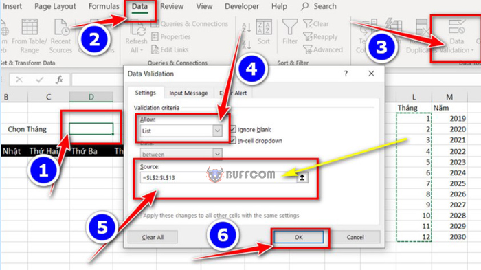
Now, create a dropdown list by clicking on the cell next to the selected month cell E3, select Data -> Data Validation -> select List in the Allow column -> click on the Source box and highlight from January to December -> ok.

How to Create an Automated Calendar in Excel

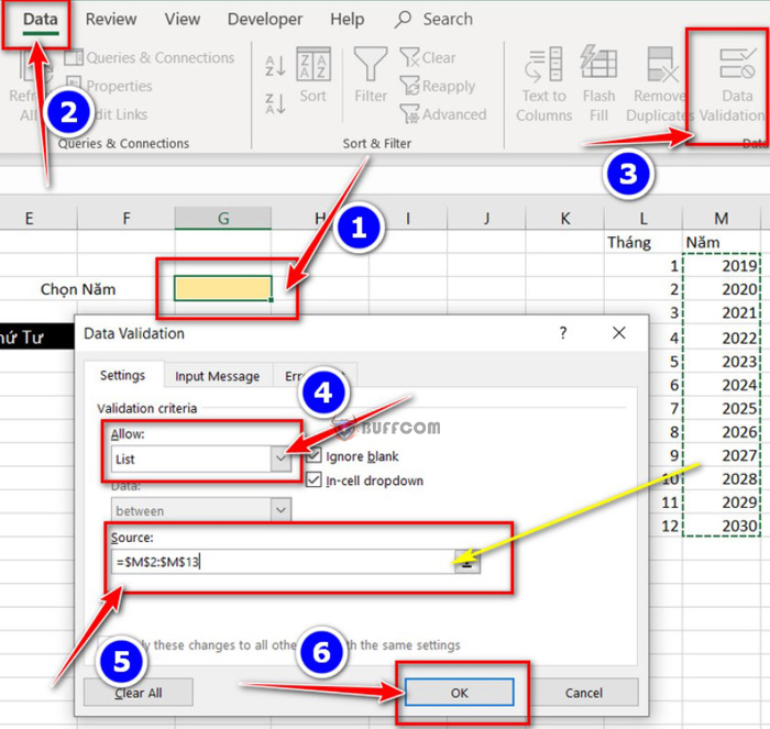
Next, to create a dropdown list for the selected year, select the cell next to the selected year list in cell G6, click on Data -> Data Validation -> select List in the Allow column -> click on the Source box and highlight from 2019 to the desired year -> ok.

How to Create an Automated Calendar in Excel

Create the calendar – Create an Automated Calendar

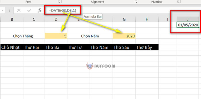
Now, to begin with May 2020, select the first day of May and year 2020 by clicking on cell J1 and enter =DATE(click on the year cell 2019; click on the May cell; enter 1, meaning the first day). Example: =DATE(G3;D3;1)

How to Create an Automated Calendar in Excel

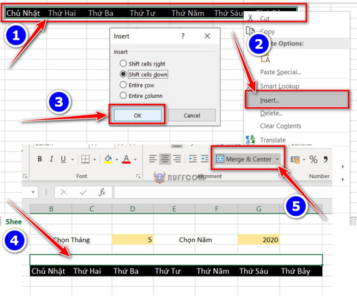
Highlight from Sunday to Monday and right-click, select Insert -> ok. Now, skip down one row and highlight the cells above from Sunday to Monday, select Merge & Center.

How to Create an Automated Calendar in Excel

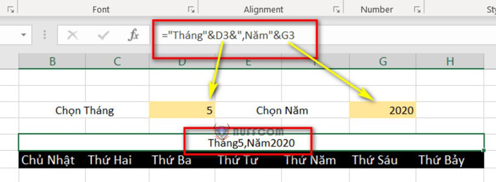
Click on the merged cell and enter =”Month” & click on the month cell & “;Year” & click on the year cell -> enter. Now, it will show the month and year that the calendar is displaying. You can also bold and color the font size.

How to Create an Automated Calendar in Excel

Before adding dates to the calendar, let me explain the Weekday function. This function returns the day of the week for the selected date, i.e., if May 1 is Friday, the Weekday function will return 6.
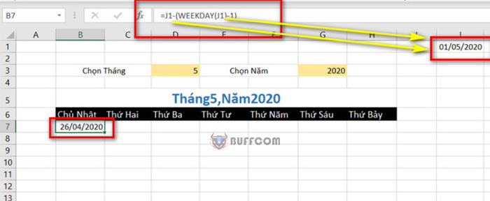
To get the closest Sunday before May, click on the cell below Sunday and enter =click on cell J1 (May 1, 2020) minus (weekday(J1)-1). And…

How to Create an Automated Calendar in Excel

Now I will create the following days. On Monday, I will use the If function with the syntax =IF<>””; click on the first Sunday date cell + 1; click on the cell above it + 7) which means if it’s not empty, the next date will be the previous date plus 1, otherwise it will be the cell above it plus 7.

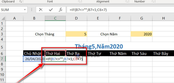
How to Create an Automated Calendar in Excel

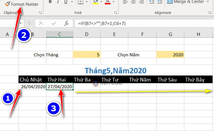
Next, click on the cell below the Sunday cell, select Format Painter -> click on the format of Monday’s date. Click on the bottom right corner of the Monday date cell and drag it to Saturday.

To create the second Sunday, click on the Monday date cell, copy it and paste it into the Sunday cell. Since the cell above it is empty, it will take the first Sunday date plus seven to get the result.

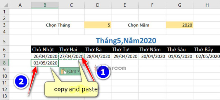
How to Create an Automated Calendar in Excel

Now, click on the bottom right corner of the date cell and drag it to the end of Saturday and down to fill all six rows like a calendar.

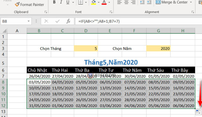
How to Create an Automated Calendar in Excel

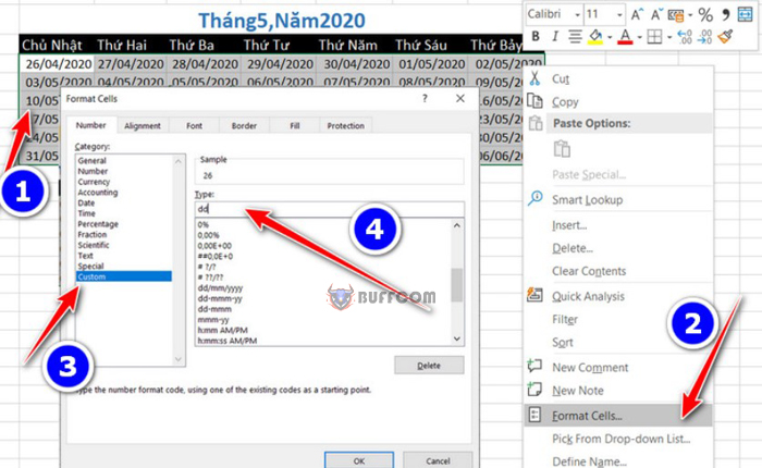
To make it look like a calendar with only dates, I will format it by selecting all the dates of the month, right-click and select Format Cells -> select Custom -> in the Type field, delete everything and type dd -> press enter. Alternatively, you can type d, and the days from 1 to 9 will not have a leading zero.

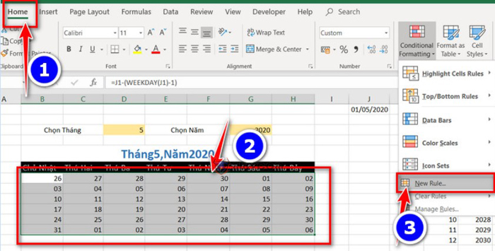
For the days that do not belong to the selected month (in this case, May), I will make them faded by selecting all the dates, clicking on Home -> Conditional Formatting -> New Rule.

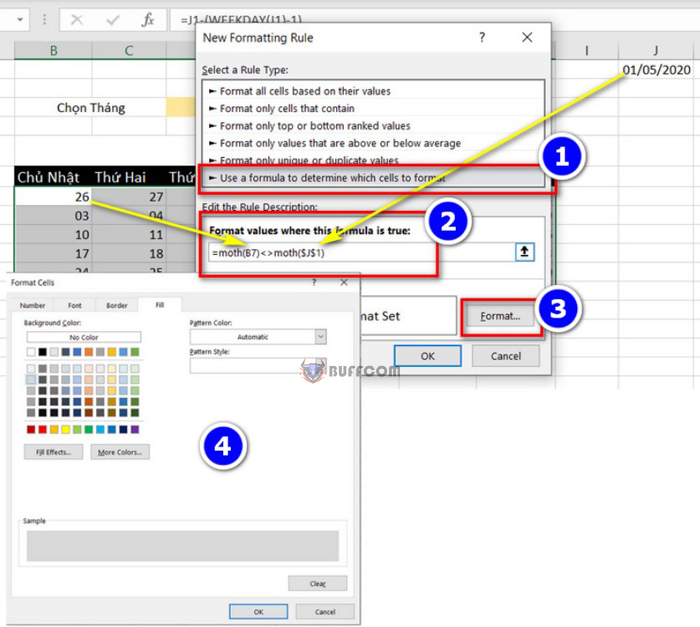
A new window appears, click on the last row in Select a rule type -> in the Format box, use the command =month(click on the first Sunday date cell, press F4 three times to remove all the previous characters)<>month(click on cell J1, which is the initial date). -> Format -> select Fill -> choose a color -> ok.

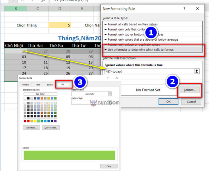
Now, I will add a condition that today’s date will be highlighted in green. Select the date range, click on Home -> Conditional Formatting -> New Rule -> select the last row in Select a rule type -> in Format, type =click on the Sunday date cell, press F4 three times =today() -> Format -> Fill -> select a color -> ok.

For Saturday and Sunday, you can change the text color to red to indicate that they are days off. In this way, you have created an automatic calendar in Excel.