3 Ways to Create Auto-Updating Dropdown Lists in Excel

3 Ways to Create Auto-Updating Dropdown Lists in Excel. Excel has a prominent feature of creating dropdown lists. With this feature, you can limit the number of entries and avoid spelling errors. Therefore, the dropdown list feature is suitable for collecting data, making it easy for readers to select items in the dropdown list.
Creating a Regular Updating Dropdown List
To create a regular dropdown list, there are two ways, and I will guide you through each method.
Creating a dropdown list by typing directly:
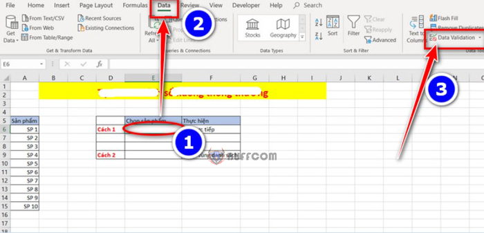
Click on the cell where you want to create a dropdown list, then select Data -> Data Validation.
3 Ways to Create Auto-Updating Dropdown Lists in Excel
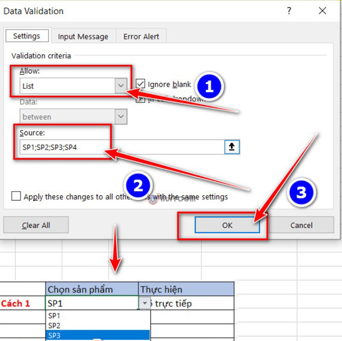
In the Allow section, select List, and then type the list directly into the Source field. For example, if you type “SP1;SP2;SP3;SP4” in the Source field, your dropdown list will have 4 items.
3 Ways to Create Auto-Updating Dropdown Lists in Excel
Creating a dropdown list using a range of data:
Click on the cell where you want to create a dropdown list, then select Data -> Data Validation.
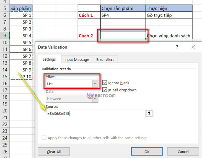
In the Allow section, select List, and then select the range of data for your dropdown list. After selecting the range of data, click OK.
3 Ways to Create Auto-Updating Dropdown Lists in Excel
These are the two basic ways to create dropdown lists in Excel. However, following the second method can save you time and reduce errors.
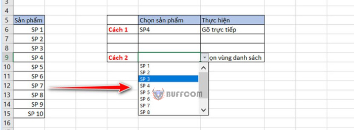
3 Ways to Create Auto-Updating Dropdown Lists in Excel
Creating a Dynamic Dropdown List
To create a dynamic dropdown list, follow these steps:
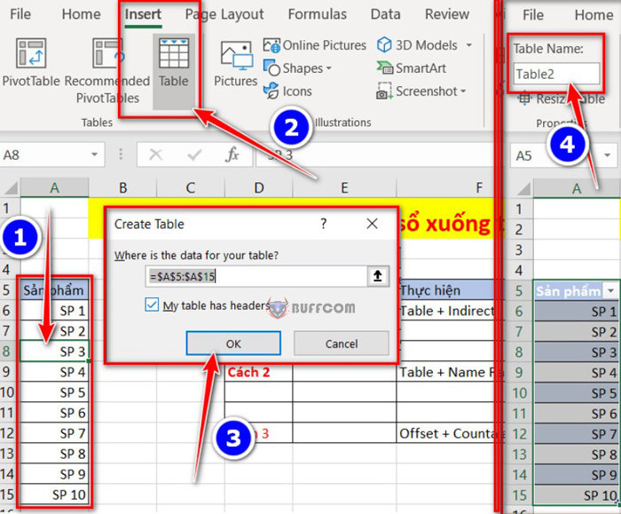
First, create a Table for the data range you want to use as a dropdown list. To do this, click on any cell within the data range, then select Insert -> Table. In the pop-up window, click OK to confirm.
In the top left corner of the screen, you can change the Table Name to whatever you want. For example, you can change it to “SP” and press Enter.
3 Ways to Create Auto-Updating Dropdown Lists in Excel
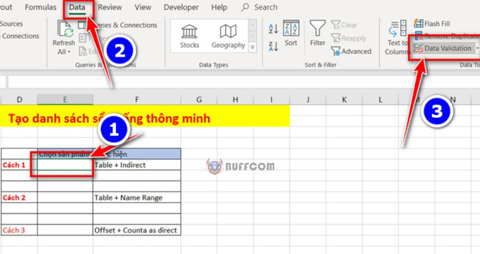
To create a dynamic dropdown list using the Table Indirect, click on the cell where you want to create the dropdown list, then select Data -> Data Validation.
3 Ways to Create Auto-Updating Dropdown Lists in Excel
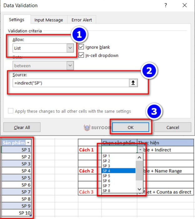
In the Allow section, select List, and then type the Indirect function in the Source field using the syntax “=Indirect(“Table name you created earlier”)”. For example, if you named your Table “SP”, then the function should be “=Indirect(“SP”)”. Press Enter to confirm.
With this smart dropdown list creation method, when you add data or a product to the Product Table, the list will automatically update.
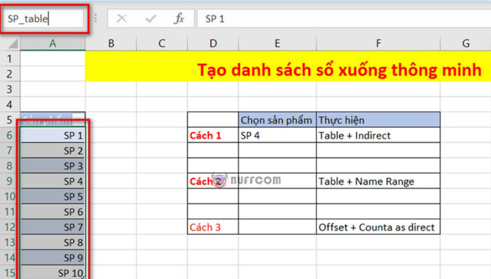
 The second method for creating a smart dropdown list is Table Name Range. Now, with the same Product Table as before, you will highlight the product names and exclude the header, then change the name in the Name Box above, for example, change it to SP_table and press Enter.
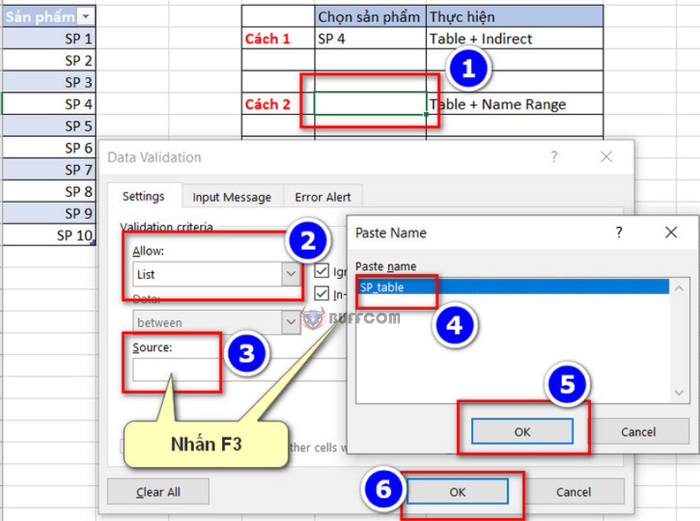
 Next, you click on the cell where you want to create the dropdown list, select Data -> Data Validation -> in the Allow section, select List -> in the Source section, press F3 and select the name of the table you just renamed -> ok.
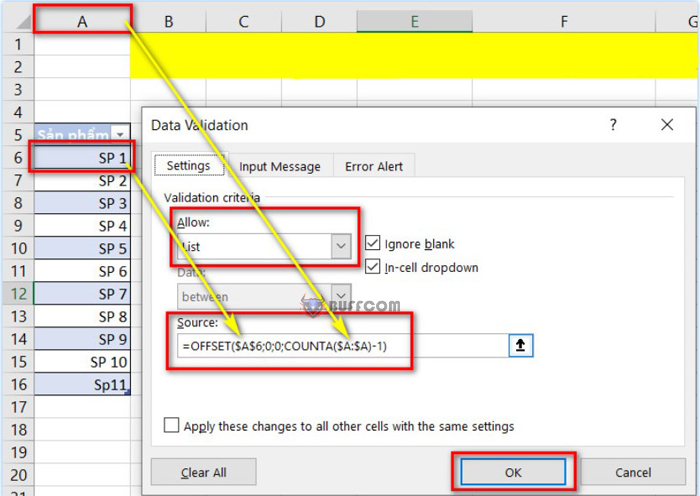
 The third method in creating a smart dropdown list is to click on the cell where you want to create the list, select Data -> Data Validation -> in the Allow section, select List -> in the Source section, use the Offset function with the syntax =Offset(click on the first product;0;0;counta(click on the column containing the products)-1) minus 1 to exclude the header of the product, for example: =OFFSET($A$6;0;0;COUNTA($A:$A)-1).
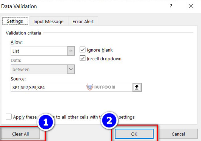
 To remove the dropdown list, you click on the cell containing the list, select Data -> Data Validation -> select Clear All -> ok. That way, the dropdown list in Excel will be removed.
