How to lock and hide formulas in Excel
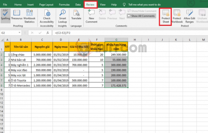
How to lock and hide formulas in Excel: Sometimes you may want to lock and hide formulas so that others can only see the results without knowing how you did it. If you don’t know how to do it, follow the steps below to learn how to lock and hide formulas in Excel.
Step 1
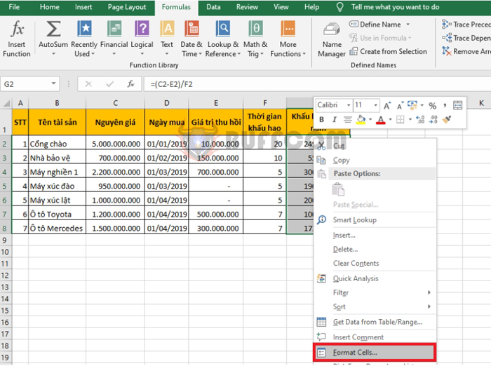
Firstly, you need to open the Excel file that you want to lock and hide formulas. Then, select the cells that you want to work on and right-click. The scroll bar will appear, and you choose the “Format Cells” option.
How to lock and hide formulas in Excel
Step 2
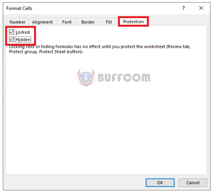
Now, the Format Cells window will appear. You select the “Protection” tab. Here, there are 2 options for you to choose from:
- Locked locks the formulas. If you choose this option, others cannot edit your formulas.
- Hidden hides the formulas. If you choose this option, the formulas will not be displayed, but others can still edit them.
If you check both Locked and Hidden options, your formulas will be locked and hidden at the same time. Finally, you click OK to complete.
How to lock and hide formulas in Excel
Step 3
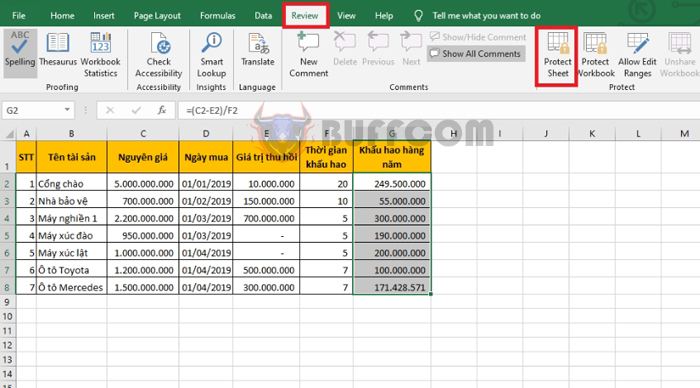
Next, you select the “Review” tab on the toolbar. Then, choose the “Protect Sheet” option.
How to lock and hide formulas in Excel
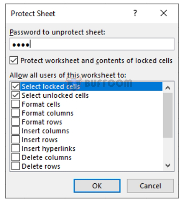
Step 4
Now, the Protect Sheet window will appear. You enter the password in the “Password to unprotect sheet” field and click OK to complete. That’s all, the formulas in the originally selected cells are now hidden and locked for editing.
How to lock and hide formulas in Excel
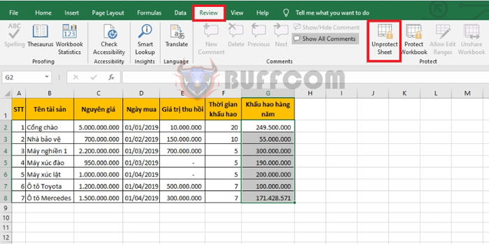
If you want to unlock these cells, you select the “Review” tab on the toolbar.
Then, choose the “Unprotect Sheet” option. The password dialog box will appear, and you enter the password and click OK to unlock the cells.
How to lock and hide formulas in Excel
Thus, the above article has instructed you on how to lock and hide formulas in Excel. We hope that this article will be useful to you during your work. Wish you success!


