Naming data ranges in Excel
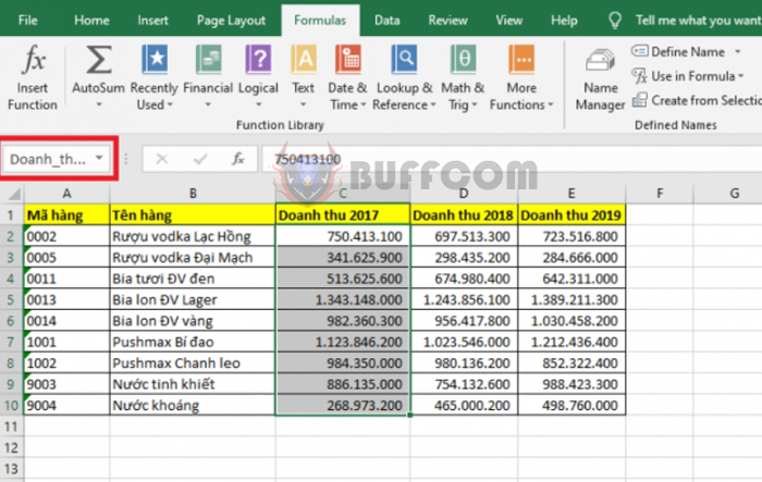
Naming data ranges in Excel: When working with Excel, if you need to refer to a data range multiple times, naming that data range can significantly reduce your operation time. Follow the article below to learn how to name data ranges in Excel.
Step 1
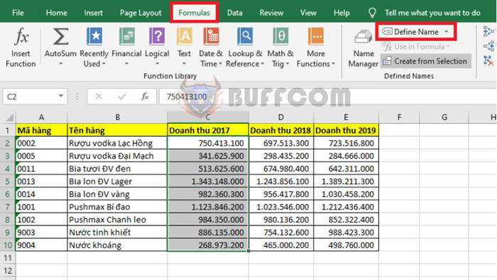
To name a data range, first, you need to select the data range you want to name. For example, in this case, if I want to name the data range containing the revenue for 2017, I will select the data range from C2 to C10. Then you select the Formulas tab on the toolbar. Next, select the Define Name option.
Naming data ranges in Excel
Step 2
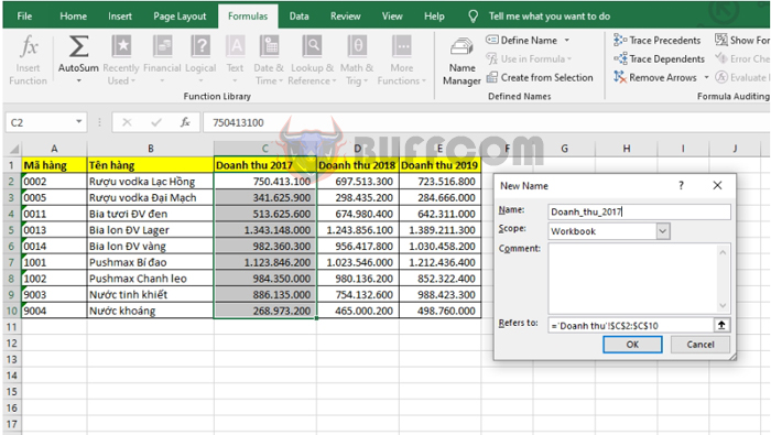
Now, the New Name window appears. You proceed to name the data range in the Name section. If you want to change the reference range, you can click on the up arrow icon in the Refers to section. Finally, click OK to complete.
Naming data ranges in Excel
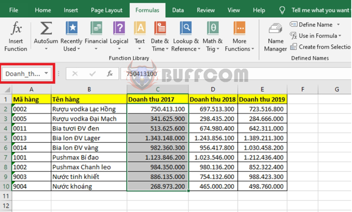
Alternatively, you can also quickly name a data range by selecting the range you want to name. Then, left-click on the Name Box next to the formula bar. Then you proceed to enter the name of the data range. Finally, press Enter to complete.
Naming data ranges in Excel
Step 3
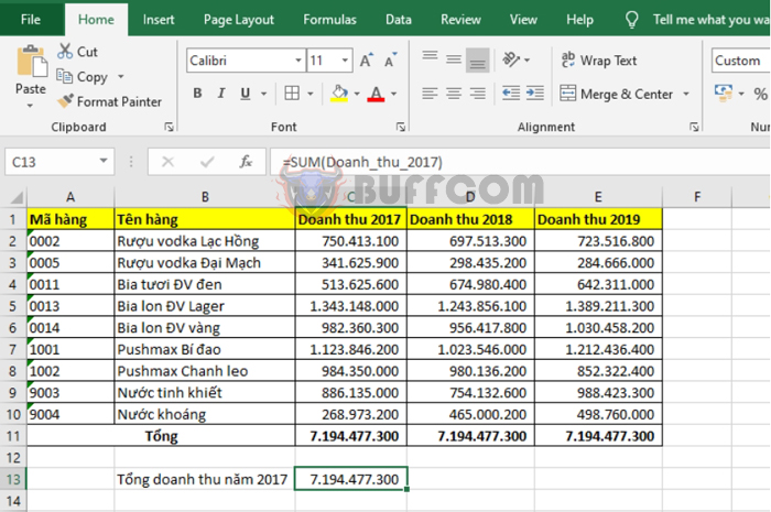
After naming the data range containing the revenue for 2017, from now on, if we need to refer to this data range, we just need to use the name Doanh_thu_2017 instead of the data range C2:C10. For example, if we need to calculate the total revenue for 2017, we use the formula: =SUM(Doanh_thu_2017) instead of =SUM(C2:C10).
Naming data ranges in Excel
Step 4
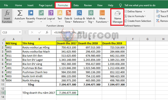
If you want to delete the name of the data range, you select the Formulas tab on the toolbar. Then left-click on the Name Manager option.
Naming data ranges in Excel
Step 5
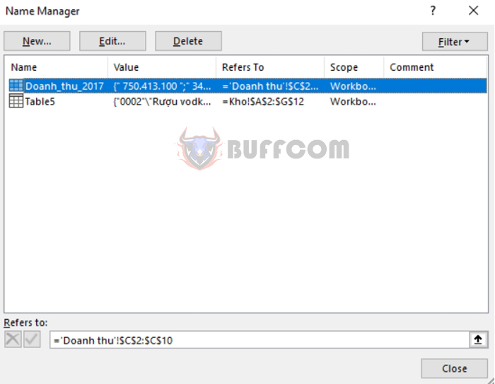
Now, the Name Manager window appears. You left-click on the name you want to delete. Then select the Delete option to delete that name. Alternatively, you can also click on Edit to edit that name.
Naming data ranges in Excel
Thus, the article has instructed you on how to name data ranges in Excel. Hopefully, the article will be useful to you in your work. Wish you success!


