Tips for Using the RANK Function to Rank Data in Excel
Tips for Using the RANK Function to Rank Data in Excel: When working with data tables in Excel and needing to classify rankings or survey growth tables, we can use the RANK function. The RANK function helps you rank data to determine which data points are high or low. Users can rank data in either descending or ascending order using the RANK function. The usage of the RANK function is relatively straightforward, similar to other basic Excel functions. The following article will guide you on how to use the RANK function to rank data in Excel.
1. RANK Function Syntax
The syntax of the function is as follows: =RANK(number, ref, [order]).
Where:
- Number: the number you want to rank within a list.
- Ref: the list of numbers. Non-numeric values in the array will be ignored.
Order: the ranking order.
- If Order is 0 or not specified, the RANK function will rank in descending order.
- If Order is 1, the RANK function will rank in ascending order.
2. How to Use the RANK Function
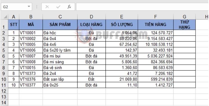
Example 1: Suppose we have a table of product prices, and we want to rank the prices.
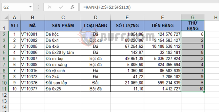
If we want to rank the prices in descending order, we enter the formula in cell G2: =RANK(F2, $F$2:$F$11, 0). Then copy the formula for the remaining cells in column G. We obtain the following result:
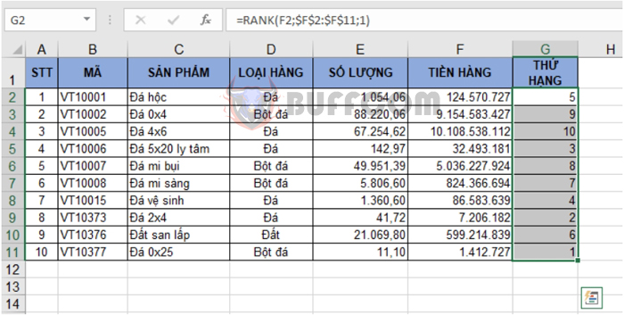
 If we want to rank the prices in ascending order, we enter the formula in cell G2: =RANK(F2, $F$2:$F$11, 1). Then copy the formula for the remaining cells in column G. We obtain the following result:
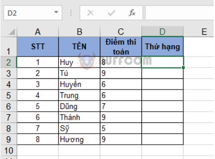
 Example 2: Suppose we have math test scores for each student, and we want to rank their scores in descending order.
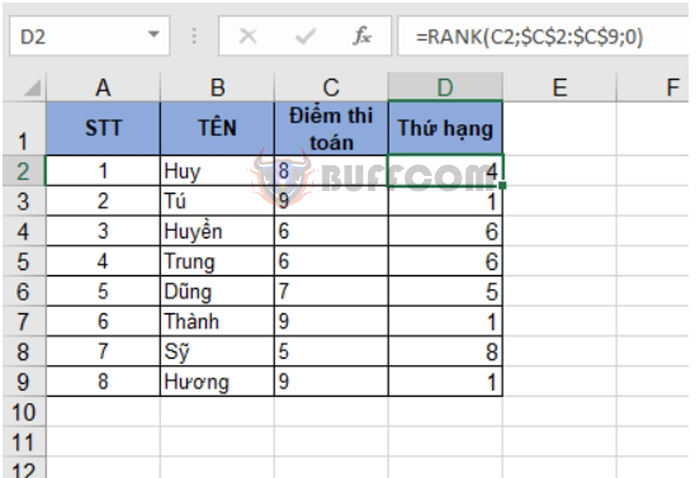
 We enter the formula in cell D2: =RANK(C2, $C$2:$C$9, 0). Then copy the formula for the remaining cells in column G. We obtain the following result:
 From the table above, we can see that Tú, Thành, and Hương are all ranked 1 because they all scored 9 points. Huyền and Trung are both ranked 6 because they both scored 6 points.
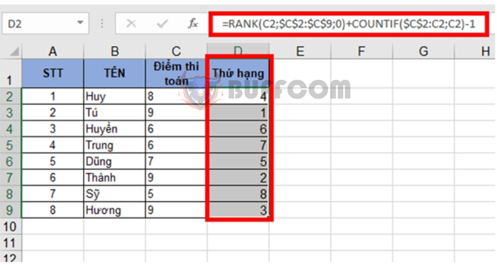
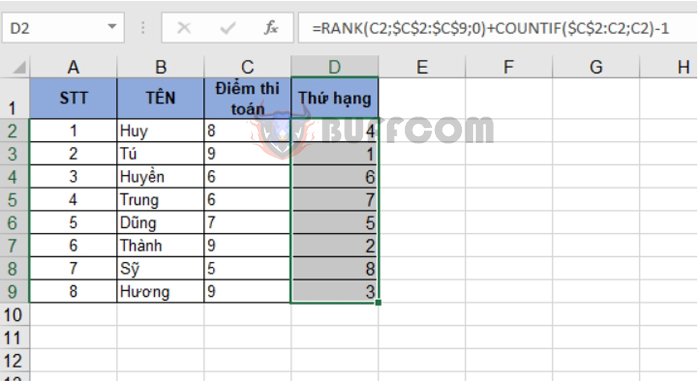
 If we don’t want to have tied ranks, we can combine the COUNTIF function with the formula to have continuous ranking without duplicate ranks.
Enter the formula in cell D2: =RANK(C2, $C$2:$C$9, 0) + COUNTIF($C$2:C2, C2) – 1. Then copy the formula for the remaining cells in column G. We obtain the following result:
Now, there are no duplicate ranks. If there are identical numbers, the number that appears first will have the earlier rank, and the number that appears later will have the later rank.
Tips for Using the RANK Function to Rank Data in Excel
That’s it! The above article has guided you on how to use the RANK function to rank data in Excel. Good luck!

