How to Perform a Two-Way Lookup in Microsoft Excel

How to Perform a Two-Way Lookup in Microsoft Excel

How to Perform a Two-Way Lookup in Microsoft Excel. This article provides instructions on how to perform a two-way lookup in Microsoft Excel.

Scenario: Suppose you need to find a value from a table without directly looking it up in the table. You require a formula that can match both a row index and a column index. This is referred to as a 2D lookup table. For example, you want to find the salary of an employee (Emp 052). In this case, the match function is used twice: once for the employee ID and once for the salary under the columns.

How to Perform a Two-Way Lookup in Microsoft Excel

Solution:

To understand the formula, it is necessary to review the following functions:

1. INDEX function
2. MATCH function

Formula:

Now, let’s create a formula using the above functions. The MATCH function will return the index of the lookup value1 in the row header field. Another MATCH function will return the index of the lookup value2 in the column header field. The index numbers will be used as input for the INDEX function to retrieve the values under the lookup value from the table data.

Generic Formula:

= INDEX(data, MATCH(lookup_value1, row_headers, 0), MATCH(lookup_value2, column_headers, 0))

• data: The array of values inside the table, excluding headers.
• lookup_value1: The value to be looked up in the row headers.
• row_headers: The row index array to be searched.
• lookup_value2: The value to be looked up in the column headers.
• column_headers: The column index array to be searched.
  

  How to Perform a Two-Way Lookup in Microsoft Excel

Example:

To better understand the above statements, let’s use the formula in an example.

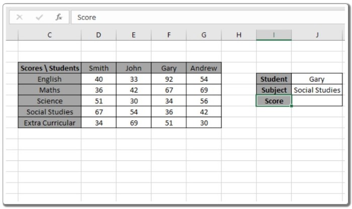
Suppose we have a list of scores obtained by students along with their subjects. We want to find the score for a specific student (Gary) and subject (Social Studies), as shown in the snapshot below.

The value1 for the student must match the row header array, and the value2 for the subject must match the column header array.

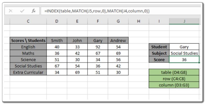
Apply the formula in cell J6: = INDEX(table, MATCH(J5, row, 0), MATCH(J4, column, 0))

How to Perform a Two-Way Lookup in Microsoft Excel

Explanation:

• The MATCH function matches the student value in cell J4 with the row header array and returns its position as 3.
• The MATCH function matches the subject value in cell J5 with the column header array and returns its position as 4.
• The INDEX function takes the row and column index numbers and searches for the matching value in the table data.
• The MATCH type argument is fixed at 0, as the formula requires an exact match.
  

  How to Perform a Two-Way Lookup in Microsoft Excel

In the above snapshot, you can see that the score obtained by student Gary in Social Studies is 36. This confirms that the formula is working correctly. For further clarification, refer to the notes below.

Now let’s use an approximate match with row headers and column headers represented as numbers. The approximate match only works with numeric values; it does not apply to text values.

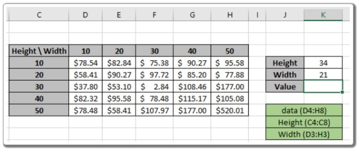
Suppose we have a price table based on the height and width of a product. We want to find the price for a specific height (34) and width (21), as shown in the snapshot below.

The value1 for the height must match the row header array, and the value2 for the width must match the column header array.

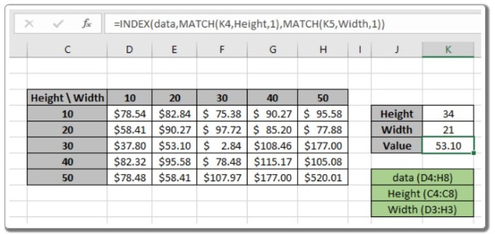
Apply the formula in cell K6: = INDEX(data, MATCH(K4, Height, 1), MATCH(K5, Width, 1))

Explanation:

• The MATCH function matches the height value in cell K4 with the row header array and returns its position as 3.
• The MATCH function matches the width value in cell K5 with the column header array and returns its position as 2.
• The INDEX function takes the row and column index numbers and searches for the matching value in the table data.
• The MATCH type argument is fixed at 1, as the formula requires an approximate match.
  

  How to Perform a Two-Way Lookup in Microsoft Excel

In the above snapshot, you can see that the price obtained for a height of 34 and width of 21 is 53.10. This confirms that the formula is working correctly. For further clarification, refer to the notes below for a better understanding.