Obtaining Relative COLUMN Index in Excel

Obtaining Relative COLUMN Index in Excel. In this article, we will explore how to obtain the relative column index in Excel. Let’s consider a scenario where we have data and need to label the index for each column. However, the data doesn’t start from the first column of the worksheet. To achieve this, we can utilize the COLUMN function along with a simple logic to calculate the column index for the data.
Obtaining Relative COLUMN Index in Excel
First, let’s understand the COLUMN function. It returns the column number of a given cell or cell reference.
Syntax: = COLUMN([cell_reference])
Note: If no argument is provided to the function, it returns the column number for the cell where the formula is used.
Now, we will create a formula using the COLUMN function and a simple logic. We want to start the index with 1, so we need to find the difference of 1 between two numbers. These two numbers will be the results of two COLUMN functions. For the rest of the table, we can extend the same formula until the last column of the data.
Generic formula: = COLUMN() – COLUMN(cell_ref)
Explanation:
- COLUMN() function returns the column number for the cell where it is used.
- To achieve the difference of 1, we use the column reference of the left adjacent cell using the COLUMN(cell_ref).
- This difference will automatically create the column index.
Obtaining Relative COLUMN Index in Excel
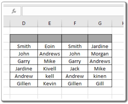
Let’s illustrate this function with an example:
Suppose we have a data table with names and values like this:
| A | B | C | D | |
| 1 | Name | Age | Sex | … |
| 2 | John | 30 | M | … |
| 3 | Jane | 25 | F | … |
| … | … | … | … | … |
We want to mark each column with its index in the given “Index Row.”
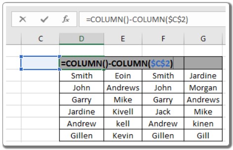
Use the following customized formula in cell D2:
Obtaining Relative COLUMN Index in Excel
= COLUMN() – COLUMN($C$2)
Explanation:
- COLUMN() will return 4, which is the corresponding column number for cell D2.
- COLUMN($C$2) will return 3, the column number for column C.
- The “$” sign fixes the cell reference to make it relative.
After entering the formula in cell D2 and pressing Enter, the result will be 1.
Now, copy the formula to the rest of the cells in the “Index Row” using the Ctrl + R shortcut or drag-right feature in Excel.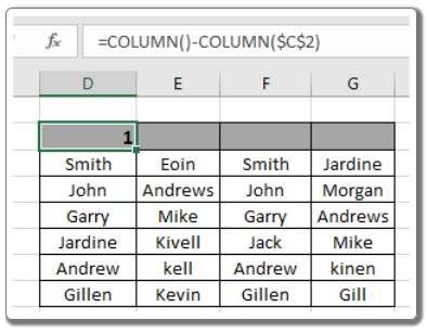
As you can see, the index column is filled with the required values.
Note: In Excel 2016 and later versions, there is an easier method to achieve the same. When you type 1 and 2 in the first and second index cells, you can select the cells and drag them right from the bottom until the column index fills automatically.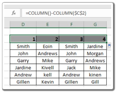
That’s it! You now know how to get the relative column index in Excel. Feel free to explore more articles on Excel cell reference functions. If you have any questions or feedback, please don’t hesitate to share them with us.

