Counting Cells with Exclusion Criteria in Excel

Counting Cells with Exclusion Criteria in Excel. In this tutorial, we will delve into the process of counting cells that meet specific criteria while excluding certain values in Excel. This technique comes in handy when we want to tally data based on specific conditions in an array. We will explore various methods to achieve this, utilizing Excel functions and wildcards for string matching.

Method 1: Using SUMPRODUCT, MATCH, and ISNA Functions

To count cells not containing certain values within a range, we can employ the following formula:

=SUMPRODUCT(—(ISNA(MATCH(range, values, 0))))

Here, ‘range’ refers to the cell array to be counted, and ‘values’ represents the array of values that should be ignored in the counting process.

Example:

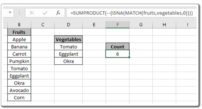
Let’s consider a scenario where column B contains fruits, and column D contains vegetables. We want to count only the fruits while disregarding any vegetables in the list.

Counting Cells with Exclusion Criteria in Excel

=SUMPRODUCT(—(ISNA(MATCH(B2:B10, D3:D5, 0))))

Explanation:

• The MATCH function attempts to find the positions where values in ‘range’ are matched with ‘values.’ If a match is not found, it returns #NA error.
• The ISNA function identifies #NA errors and returns TRUE for each occurrence and FALSE otherwise.
• The double unary operator (–) converts TRUE to 1 and FALSE to 0.
• Finally, the SUMPRODUCT function sums up all the resulting 1s, yielding the count of cells where values are not considered.
  

  Counting Cells with Exclusion Criteria in Excel

Method 2: Utilizing the COUNTIFS Function

Another method involves using the COUNTIFS function, which allows us to count cells based on multiple criteria. We can construct the formula as follows:

=COUNTIFS(range, “<>value1”, range, “<>value2”, …)

Here, ‘range’ refers to the cell array to be counted, and ‘value1’, ‘value2’, etc., represent the values that should be ignored in the counting process.

Example:

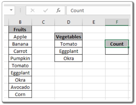
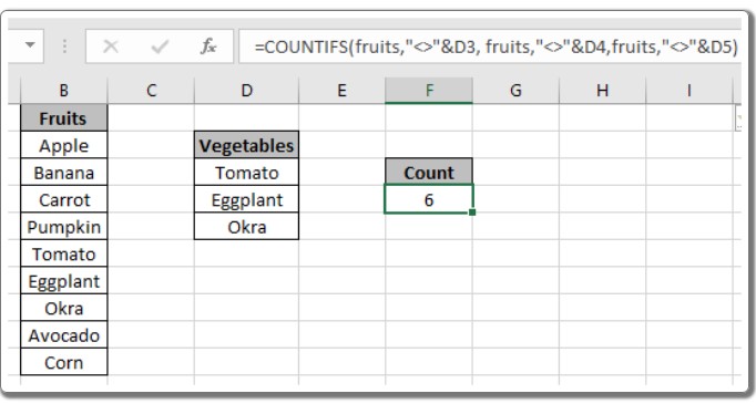
Let’s consider the same scenario, where column B contains fruits, and column D contains vegetables. We want to count only the fruits while disregarding any vegetables in the list.

=COUNTIFS(B2:B10, “<>”&D3, B2:B10, “<>”&D4, B2:B10, “<>”&D5)

Counting Cells with Exclusion Criteria in Excel

Explanation:

• The formula checks each cell in the ‘range’ against individual ‘values’ and returns the count of cells that meet the criteria (not equal to the specified values).
• The “<>” operator signifies “not equals to.”
• The “&” operator concatenates the operator with the value referenced by the cell.
  

  Counting Cells with Exclusion Criteria in Excel

Method 3: Using COUNTA and SUMPRODUCT with COUNTIF

Another approach involves using the COUNTA function to calculate the count of non-empty cells in a range and then subtracting the count of cells containing specific values using COUNTIF.

=COUNTA(range) – SUMPRODUCT(COUNTIF(range, values))

Here, ‘range’ refers to the cell array to be counted, and ‘values’ represents the array of values that should be ignored in the counting process.

Example:

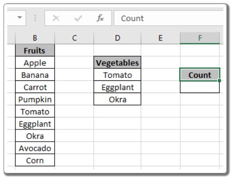
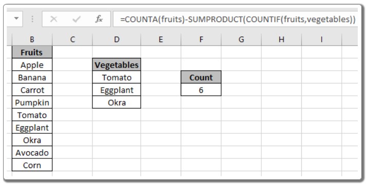
Let’s consider the same scenario with fruits in column B and vegetables in column D. We want to count only the fruits while disregarding any vegetables in the list.

=COUNTA(B2:B10) – SUMPRODUCT(COUNTIF(B2:B10, D3:D5))

Counting Cells with Exclusion Criteria in Excel

Explanation:

• The COUNTIF function counts the occurrences of ‘values’ (vegetables) in the ‘range’ (fruits).
• SUMPRODUCT sums up all the counts obtained from COUNTIF.
• COUNTA calculates the count of non-empty cells in the ‘range.’
• Subtracting the count of vegetable cells from the total count gives us the desired result: the count of cells (fruits) without the specified values (vegetables).
  

  Counting Cells with Exclusion Criteria in Excel

Conclusion:

By employing these various methods, you can efficiently count cells in Excel while excluding specific values based on your requirements. These techniques can prove valuable in data analysis and processing. Feel free to explore further Excel count functions and apply them to your tasks to enhance your spreadsheet capabilities. Should you have any questions or feedback regarding this article, please do not hesitate to share them with us.