Advanced Techniques for Conditional Formatting in Excel
Advanced Techniques for Conditional Formatting in Excel
Advanced Techniques for Conditional Formatting in Excel. In this guide, we will delve into advanced techniques for utilizing Conditional Formatting in Microsoft Excel.
Advanced Techniques for Conditional Formatting in Excel
Scenario:
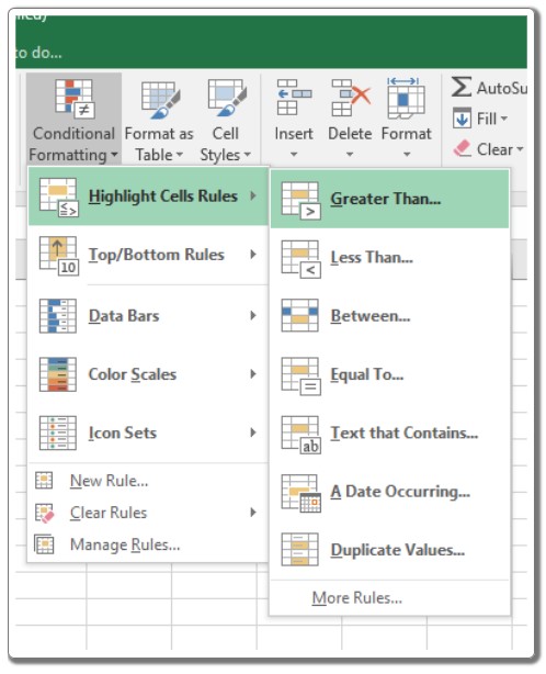
Microsoft Excel boasts numerous powerful capabilities that may not be immediately apparent. One such feature is Conditional Formatting, a tool employed to format cells or ranges based on specific conditions. This tool can be applied to cell values or formulas. For instance, if a cell contains a formula, you can define formatting conditions using “Conditional Formatting,” or if a range contains values, you can specify conditions using formulas to highlight those values.
Advanced Techniques for Conditional Formatting in Excel
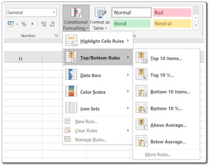
There exists a multitude of ways to leverage “Conditional Formatting” in our data. It can be utilized to display numbers in ascending or descending order, based on specific values, certain numbers, particular dates, and more. Furthermore, you can emphasize cells by filling them with color, changing font color, employing data bars, color scales, and icon sets.
Exploring Further Conditional Formatting Techniques in Excel:
Below are some common scenarios where Conditional Formatting proves invaluable for highlighting cells based on specific conditions in Excel:
1. Highlighting a Cell Dependent on Another Cell:
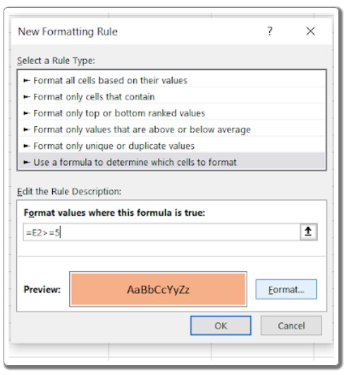
Conditional formatting involves establishing conditions where one cell’s format depends on another cell’s value. For instance, you might want to format IDs if the number of nights spent exceeds or equals 5. Follow these steps:

Advanced Techniques for Conditional Formatting in Excel
Select the ID column.
Navigate to Conditional Formatting > New Rule.
Choose “Use a formula to determine which cells to format.”
Use the formula: =E2>=5.
Select a formatting style, like changing the background color to Orange, for cells satisfying the condition.
Advanced Techniques for Conditional Formatting in Excel
2. Formatting Based on Date Columns:
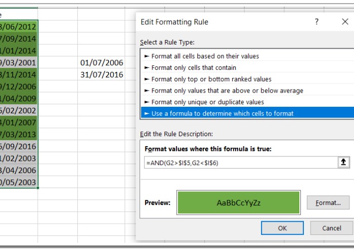
Dates are treated as serial numbers in Excel. To format cells based on dates, treat them as numerical values or use cell references. For instance, to format date cells falling between two given dates:

Advanced Techniques for Conditional Formatting in Excel
Select the date values.
Go to Conditional Formatting > New Rule.
Choose “Use a formula to determine which cells to format.”
Use the formula: =AND(G2>$I$5,G2<$I$6) (assuming the dates are in column G and the range’s start and end dates are in cells I5 and I6).
3. Hiding Zeros Using Conditional Formatting:
Concealing zero values within a table is accomplished by making them visually blend with the background. For instance:
Advanced Techniques for Conditional Formatting in Excel
Select the data.
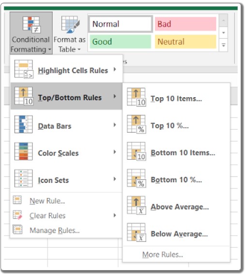
Navigate to Conditional Formatting > Highlight Cells Rules > Equal To.
Set the value to 0.
Format the font color to match the background color or vice versa.
Advanced Techniques for Conditional Formatting in Excel
These advanced techniques showcase the versatility of Conditional Formatting within Excel. This feature not only simplifies data interpretation but also enhances data visualization. By understanding and implementing these techniques, you can harness the power of Conditional Formatting to its fullest extent.


