How to Calculate the Average of the Top 5 Values in Excel


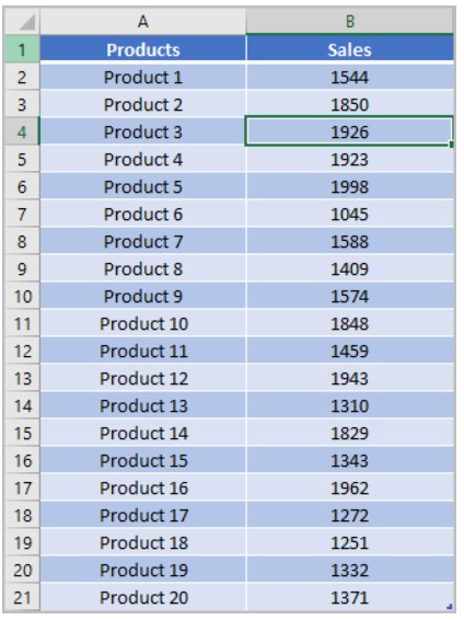
Suppose you have a list of 20 products in your company, along with the monthly sales data for each of the products. If you want to find the average of the top 5 products based on their sales data, you can follow these steps:
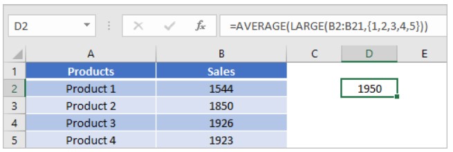
Use the following formula to calculate the average of the top 5 values:
- =AVERAGE(LARGE(B2:B21,{1,2,3,4,5}))

- The formula combines the LARGE and AVERAGE functions. Let’s break it down to understand how it works.
LARGE Function:
The LARGE function allows you to find the nth largest value from a range of data. In this case, we want to find the top 5 values. To achieve this, we use an array as the second argument of the LARGE function:
{1,2,3,4,5}
By entering this array, the LARGE function returns an array of the top 5 from the data range (B2:B21).
AVERAGE Function:
The AVERAGE function then calculates the average of the returned by the LARGE function. It takes the array of the top 5 as its argument and provides the average result.
Important Note:

When entering the formula, remember to press CTRL + SHIFT + ENTER instead of just pressing ENTER. This ensures that the formula is treated as an array formula by Excel.
By following these steps, you will obtain the average of the top 5 values from the given data range.


