How to Display Negative Numbers in Parentheses in Excel
How to Display Negative Numbers in Parentheses in Excel. To make negative numbers look neater and more presentable while processing data, in this article, I will guide you on how to display negative numbers in parentheses in Excel. Let’s dive into the article!
Example of display negative numbers in parentheses
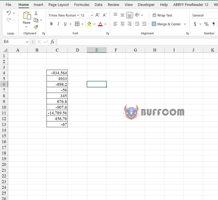
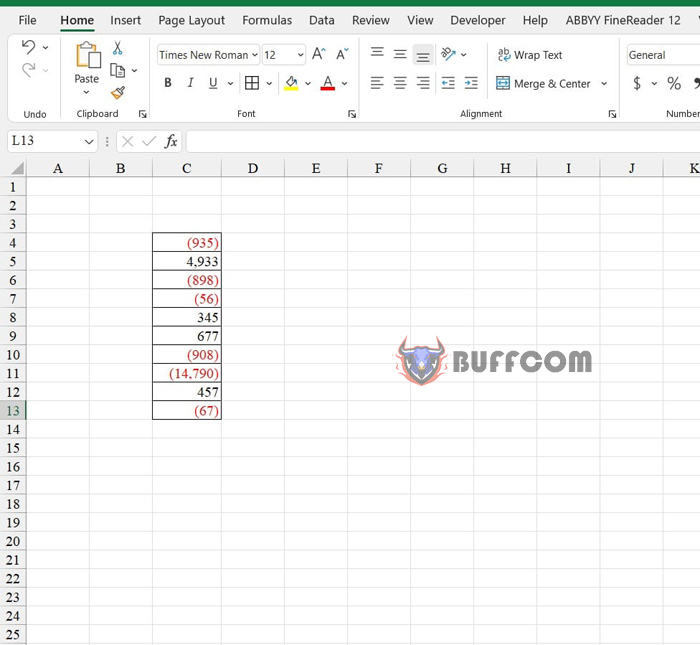
Consider the data below:
How to Display Negative Numbers in Parentheses in Excel
The requirement is to display negative numbers in a shortened format enclosed within parentheses and with red font. To achieve this, follow these steps:
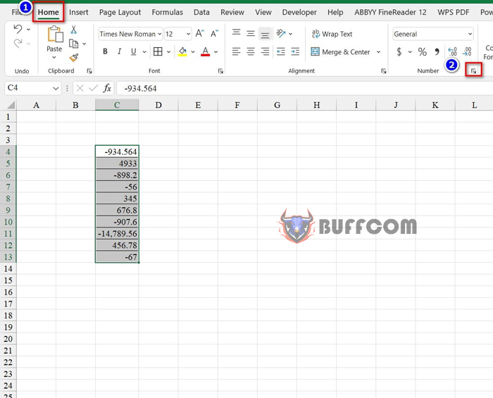
Step 1: Select the data range
Step 2: Go to the Home tab, click the arrow on the right of the Number group.
Step 3: In the Format Cells dialog box, select the Custom category, and in the Type box, enter “#,##0;red”.
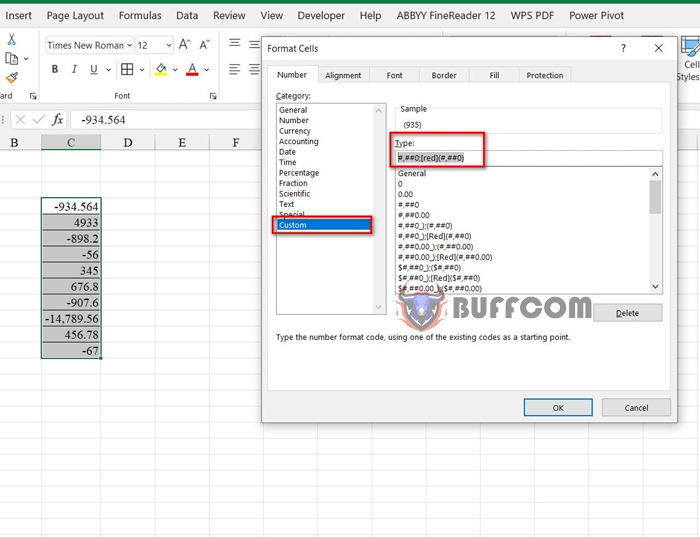
Step 4: Click OK to complete.
To modify the display format: Select the data range, and then click the arrow next to the Number group again. In the Format Cells dialog box, you can modify the Type according to your requirements.
That’s it! I have just guided you on how to display negative numbers in parentheses in Excel. I hope you find this article useful, and if you do, don’t forget to rate it below!


