3 Easy Ways to Get Month Names from Dates in Excel
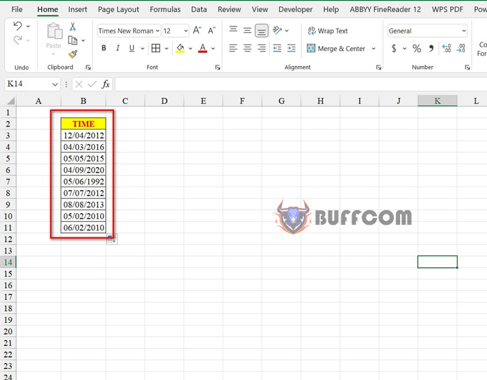
3 Easy Ways to Get Month Names from Dates in Excel. When processing a time column, you may want to extract the month or display the month name from that date. In this article, I will show you 3 easy ways to get the month name from a date in Excel. Let’s take a look at the following example data:
3 Easy Ways to Get Month Names from Dates in Excel
To get the month name based on the above data, you have three methods as follows:
Method 1: Get the month names from Custom Number Format
Steps to perform:
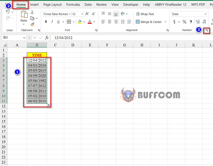
Step 1: Select the data range containing the time you want to display the month name.
Step 2: Go to the Home tab, click on the arrow next to the Number group.
3 Easy Ways to Get Month Names from Dates in Excel
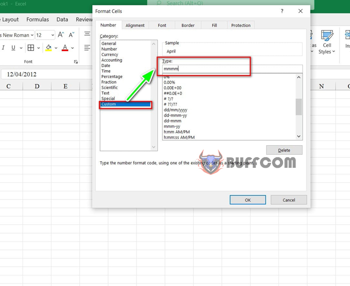
Step 3: The Format Cells dialog box appears. Choose Custom and type “mmmm” in the Type box.
3 Easy Ways to Get Month Names from Dates in Excel
Step 4: Press OK to display the result.
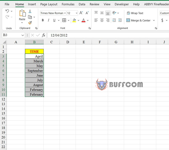
3 Easy Ways to Get Month Names from Dates in Excel
Method 2: Get the month names from the Text function
First, you select the cell to display the month name. Next, you enter the following formula: =TEXT(B3,”mmmm”)
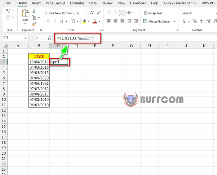
3 Easy Ways to Get Month Names from Dates in Excel
Finally, to display the remaining cells, you also select from the first cell to the last row and press Ctrl + D.
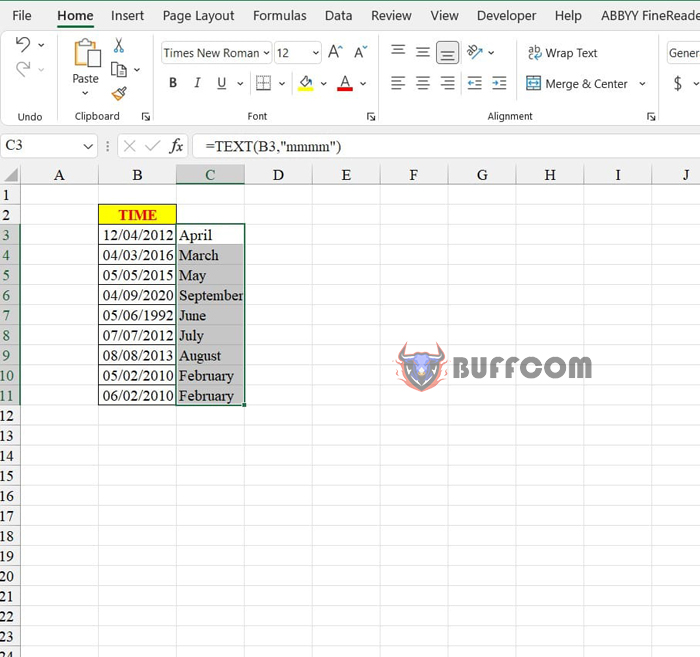
3 Easy Ways to Get Month Names from Dates in Excel
Moreover, to calculate the quarter based on the month, you use the following formula: =ROUNDUP(MONTH(B3)/3,0).
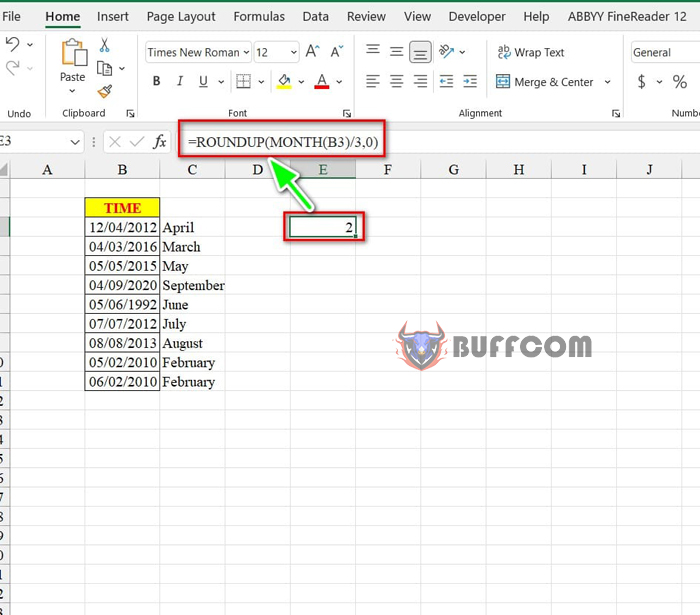
3 Easy Ways to Get Month Names from Dates in Excel
Method 3: Get the month names using Power Query
Steps to perform:
Step 1: Select any cell in the data table, then go to the Insert tab, select Table, and click OK to create a data table.
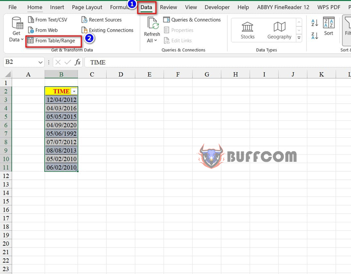
Step 2: In the data, go to the Data tab, select From Table/Range
3 Easy Ways to Get Month Names from Dates in Excel
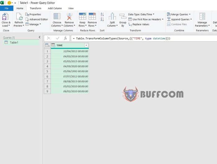
Step 3: The Power Query interface appears.
3 Easy Ways to Get Month Names from Dates in Excel
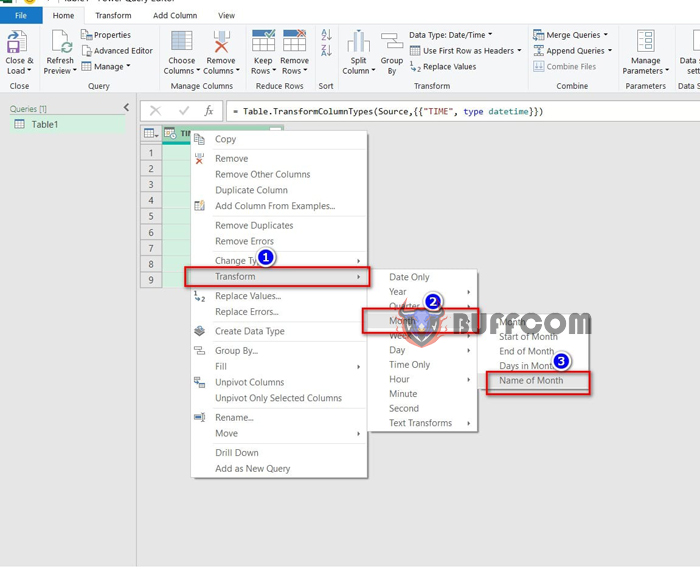
Step 4: Right-click on the column header, select Transform, then select Month, and then select Name of Month.
3 Easy Ways to Get Month Names from Dates in Excel
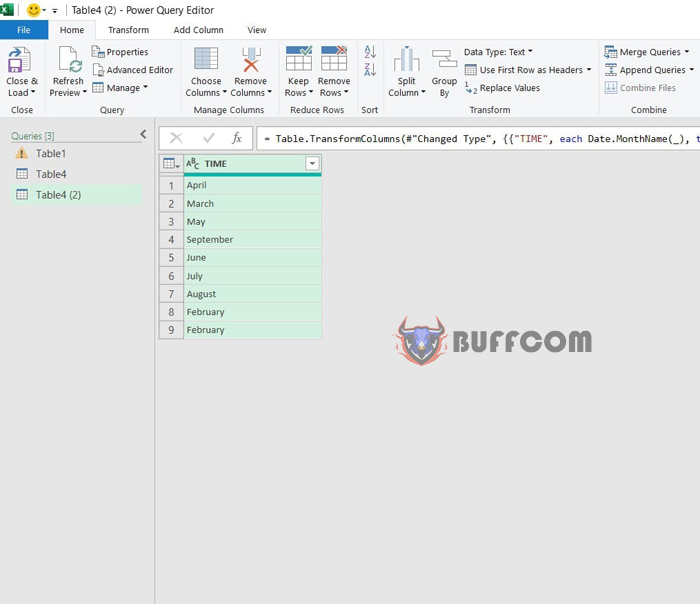
Step 5: The result is displayed.
3 Easy Ways to Get Month Names from Dates in Excel
Step 6: To exit the Power Query interface, go to the Home tab and click on Close & Load.
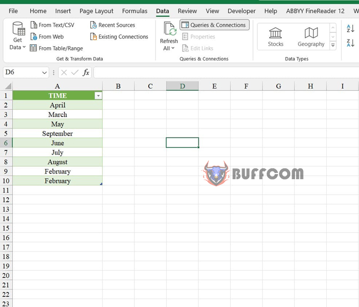
3 Easy Ways to Get Month Names from Dates in Excel
So, I have just shown you 3 ways to display month names from dates in Excel. I hope you can successfully apply these methods. If you find this article helpful, don’t forget to rate it below! Best regards from Buffcom.


