How to create lists in Excel and Google Sheets quickly and easily

Excel and Google Sheets are powerful tools that help users optimize their work processes. They provide many features that allow users to present and process their spreadsheets more efficiently. Among these features, creating lists in Excel is commonly used to help you create a dropdown list of options that you can select directly without having to enter it. So how do you create a dropdown list in Excel? Let’s find out in this article!
How to create and customize dropdown lists in Excel
Creating a dropdown list in Excel, also known as a list box in spreadsheet cells, can be especially useful when users want to create customized categories. This Drop List typically includes data such as gender, occupation, location, title, etc. Using dropdown lists will save you time and effort by avoiding the need to enter duplicate data.
How to create a list in Excel
To create a list box in Excel, you can follow these steps:
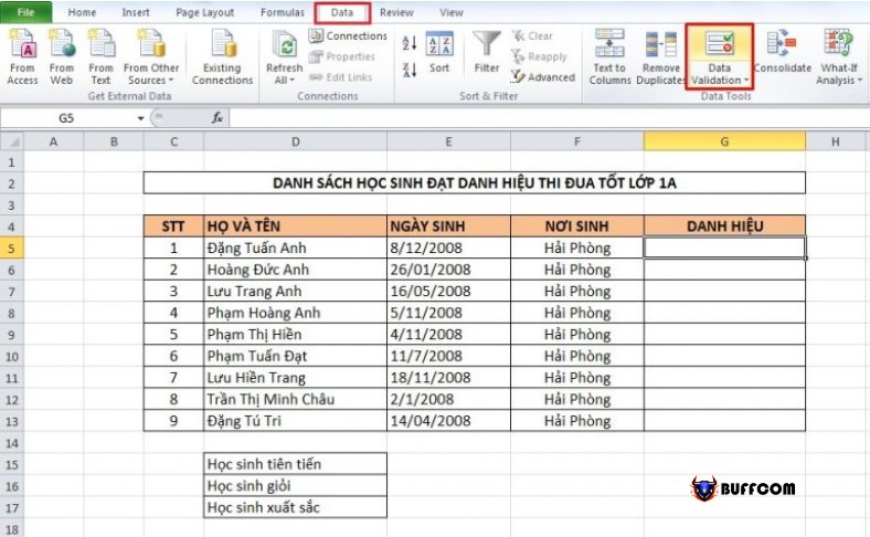
Step 1: Enter the data you want to create a dropdown list for in an empty area on the worksheet. Select the cell where you want to create the dropdown list in Excel. Then select “Data” and choose “Data Validation.”
How to create lists in Excel and Google Sheets
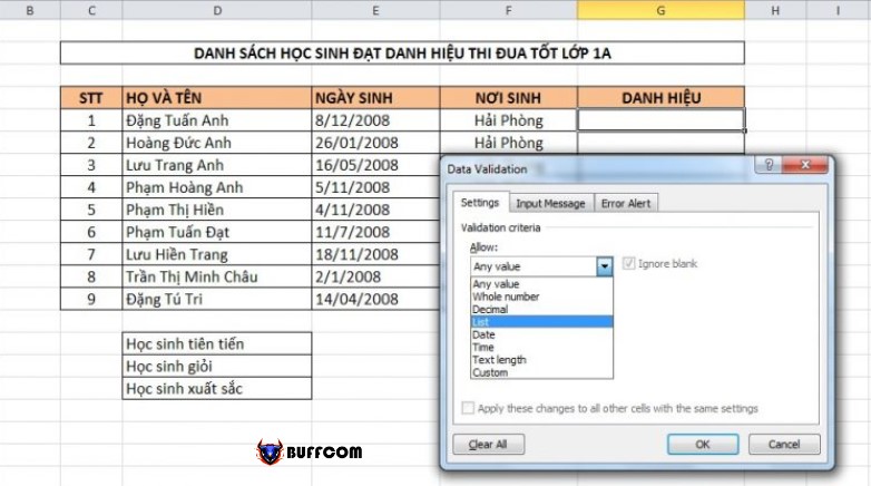
Step 2: The Data Validation dialog box will appear. On the “Settings” tab, choose “List” in the “Allow” field.
How to create lists in Excel and Google Sheets
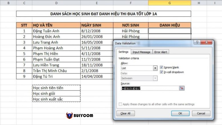
Next, under “Sources,” select the range of dropdown data that you have created on the worksheet.
How to create lists in Excel and Google Sheets
Step 3: Finally, click OK to create the dropdown list in Excel for the cell you have selected.
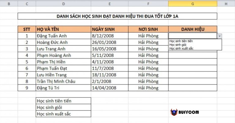
How to create lists in Excel and Google Sheets
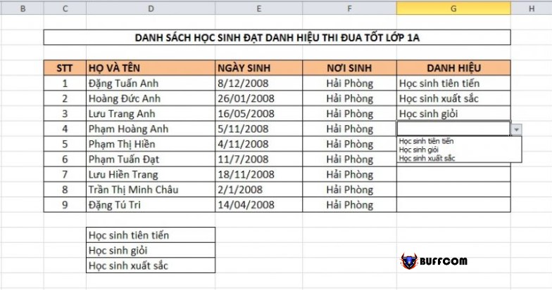
In addition, to copy the dropdown list to other cells in the column, simply drag down to receive the same result. At this point, in the worksheet cells, you only need to select the appropriate data without having to enter them again.
How to create lists in Excel and Google Sheets
Furthermore, if your worksheet requires multiple different dropdown lists (with different attribute data ranges), you will need to name the dropdown range to manage and use them more conveniently. For example, if you want to edit the data range or edit the name or delete the Drop List. To name the dropdown list, follow these steps:
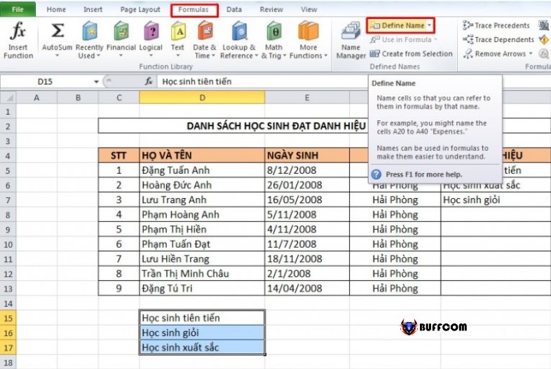
Select the data range you want to create and name the dropdown list.
Go to the Formulas section. Then select Define Name.
How to create lists in Excel and Google Sheets
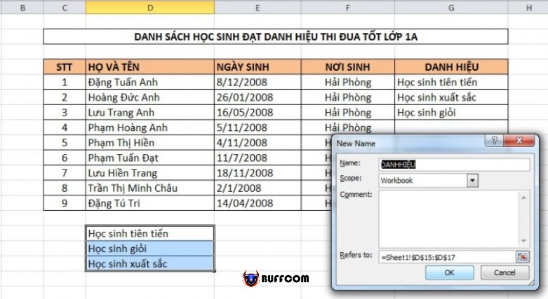
Enter the name for the data range in the Name field. Note that you need to name the data range the same as the column name of the data but without spaces between the characters.
How to create lists in Excel and Google Sheets
Click OK to complete.
How to Customize Drop-Down List in Excel
Copy and Paste Drop List
Unlike regular data in a worksheet, to copy the cells containing a drop-down list to another location, follow these steps:
Step 1: Select the cell containing the drop-down list format. Right-click and select Copy (or press Ctrl + C).
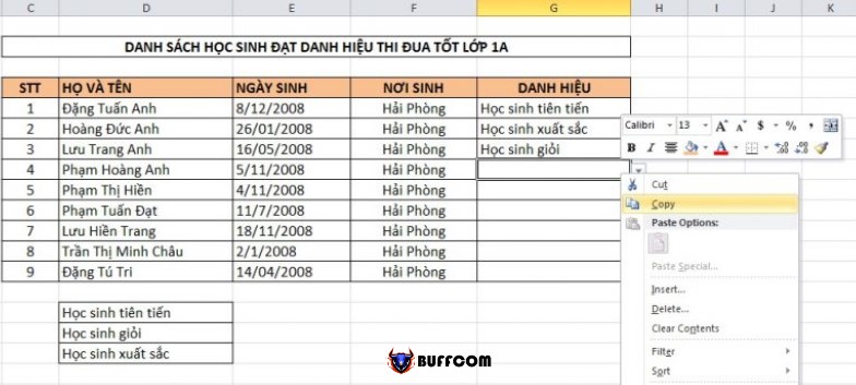
How to create lists in Excel and Google Sheets
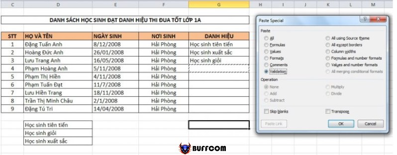
Step 2: Select the location you want to move the drop-down list to. Right-click on that cell and select Paste Special…
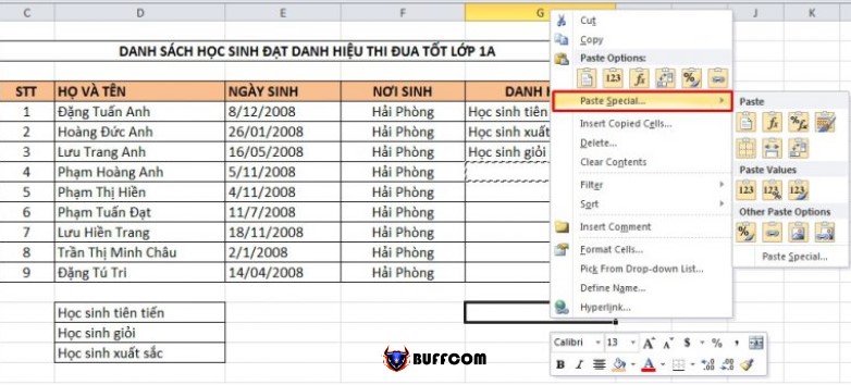
How to create lists in Excel and Google Sheets
Step 3: In the Paste section, check Validation. Then click OK.
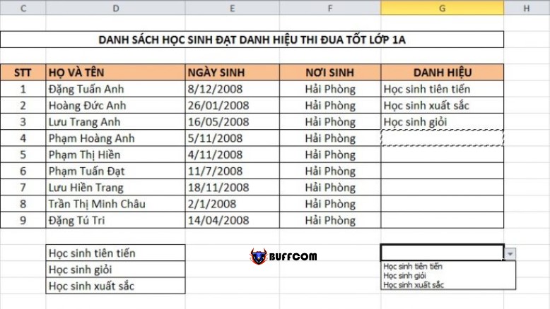
How to create lists in Excel and Google Sheets
Edit Data Range for Drop-Down List
To change or edit the data range for a drop-down list, follow these steps:
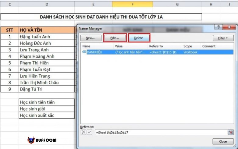
Step 1: Go to the Formulas tab and select Name Manager.
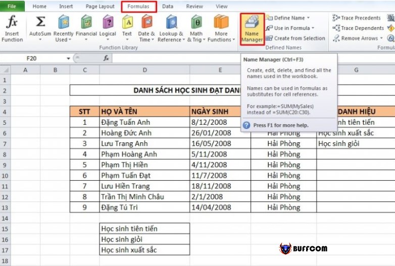
How to create lists in Excel and Google Sheets
Step 2: The Name Manager dialog box appears, where you can edit or delete the data range in the corresponding Edit and Delete sections.
How to create lists in Excel and Google Sheets
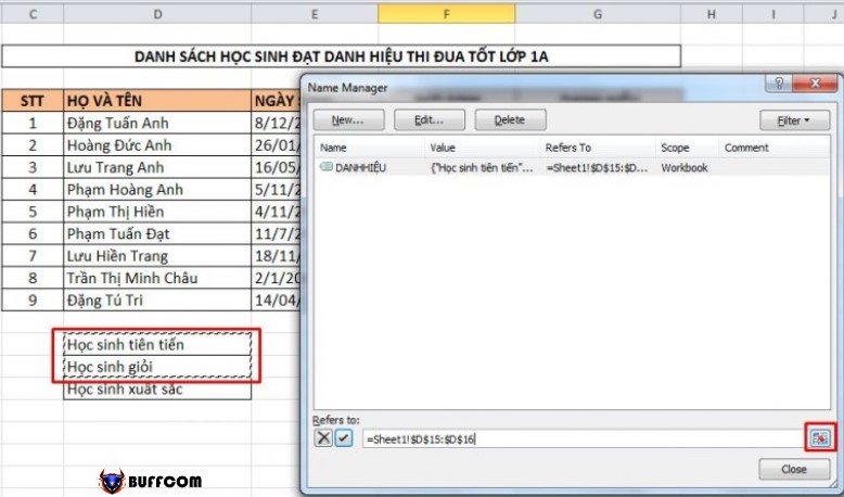
Or if you want to change the data range, select the upward arrow symbol and reference the data range you want to change.
How to create lists in Excel and Google Sheets
Delete Drop-Down List in Excel
To delete a drop-down list, follow these steps:
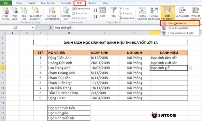
Step 1: Select the cell with the list in Excel > Click on the Data tab > Select Data Validation.
How to create lists in Excel and Google Sheets
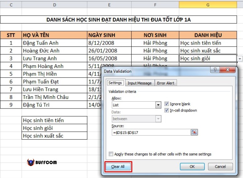
Step 2: Click on Clear All. Finally, click OK to complete deleting the drop-down list.
How to create lists in Excel and Google Sheets
How to create a Drop List in Google Sheets
Google Sheets is the online version of Excel. The features and tools in these two applications are similar, except that Google Sheets will automatically save your data on cloud storage. Meanwhile, with Microsoft Excel, you have to save the file after each edit, and it will also consume a portion of your computer’s resources for storage. Therefore, with the advantages that Google Sheets possesses, this tool is increasingly popular and widely used.
Creating a list in Google Sheets with available data
Creating a drop list in Google Sheets is similar to Excel, and you can do it as follows:
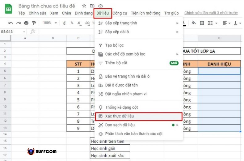
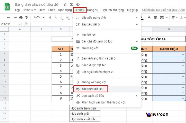
Step 1: Select one or more cells where you want to create the Drop List. Then select Data > Data validation.
How to create lists in Excel and Google Sheets
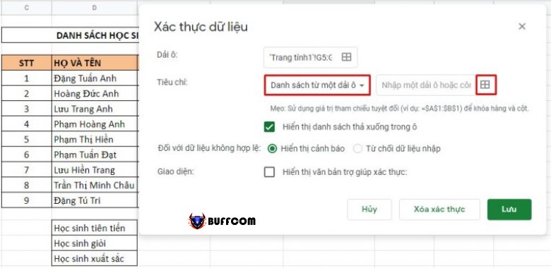
Step 2: In the “Criteria” section, select “List from a range of cells.” Then, click on the grid icon next to it.
How to create lists in Excel and Google Sheets
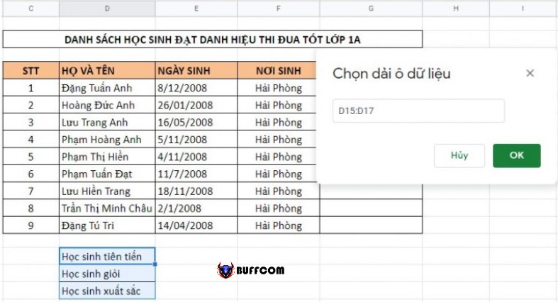
Step 3: Select the range of data you want to create a drop-down list from and click OK.
How to create lists in Excel and Google Sheets
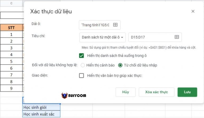
Step 4: In the “Invalid data” section, check the “Reject input” box.
How to create lists in Excel and Google Sheets
Step 5: Click Save to create the list in the online version of Excel.
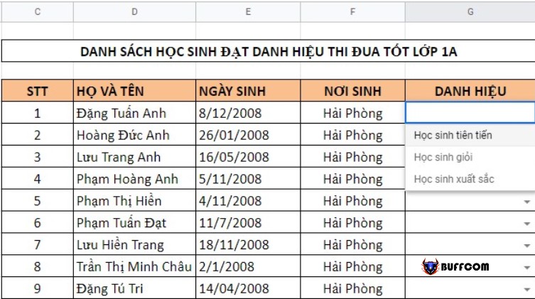
How to create lists in Excel and Google Sheets
Creating a list in Google Sheets by manually entering data
In addition to using pre-entered data on the spreadsheet, you can also directly enter this data when setting up the Drop List as follows:
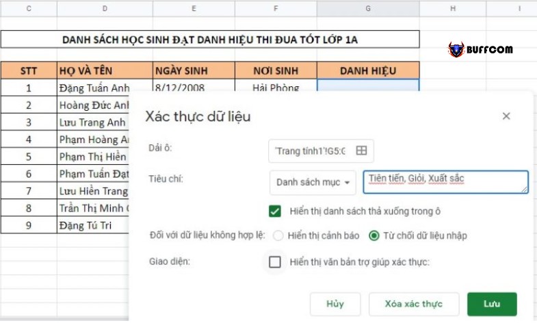
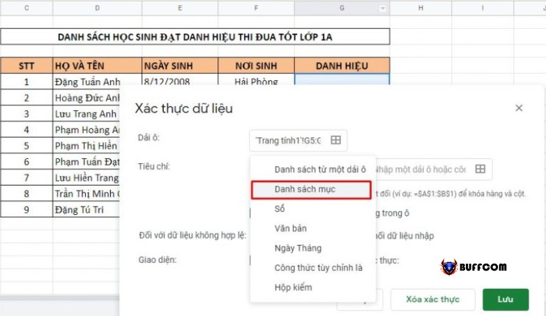
Step 1: Similarly, select one or more cells to create the drop-down list. Then select Data > Data validation.
Step 2: In the “Criteria” section, select “List of items.” Then, in the box next to it, enter the numerical or text data, and these values must be separated by commas.
How to create lists in Excel and Google Sheets
Check the “Show drop-down list in cell” and select “Reject input” in the “Invalid data” section.
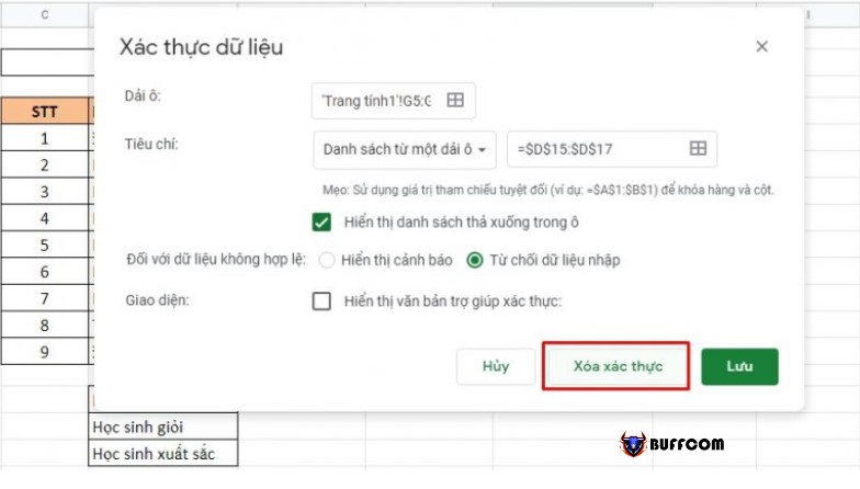
In addition, if you want to delete cells that have been created with a Drop List, you can quickly do so by selecting the cells with the Drop List format that has been created > Select Data > Select Data validation > Press Delete validation. Then all cells containing the drop-down list will be completely deleted.
How to create lists in Excel and Google Sheets
Step 3: Finally, click Save to complete.
Above is a detailed guide on how to create a list in Excel and Google Sheets. Hopefully, with these sharing, users can successfully create drop-down lists to optimize their work. Good luck!

