How to Efficiently Use Excel Styles

Styles are often associated with Microsoft Word, but you may be surprised to learn that Microsoft Excel also utilizes styles, albeit in a different manner. Excel styles are simpler to use compared to Word styles. If you haven’t been using them because you find them complicated, it’s time to reconsider. In this article, I will introduce you to Excel styles and demonstrate how they can enhance your efficiency in Excel.

What is a Microsoft Excel Style?

If you’re unfamiliar with styles, you might wonder what makes them special. The simple answer is that they help you work more efficiently. A style is a collection of formats that can be applied simultaneously. For example, you might want all input cells to have a green background with white font. By using a style, you can apply both formats at once. This may not sound significant, but there’s more to it. If you decide to change the format for input cells, you don’t need to modify each cell individually. Simply modify the style, and all input cells will automatically update. That’s true efficiency in action.

Styles in Microsoft Excel

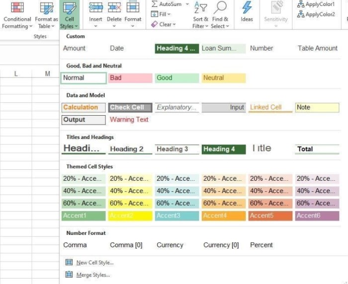
Styles in Excel (and other Office 365 apps) are not as apparent as they are in Word. You can find styles in the Styles group on the Home tab, under Format a Table and Cell Styles. In this article, we will focus on working with the Cell Styles option. As shown in Figure A, the dropdown offers various built-in cell styles.

Figure A

How to Efficiently Use Excel Styles

You may not be aware, but you are already using a style called “Normal” – this is the default formatting you see when entering data on a new sheet. Towards the bottom of the gallery (Figure A), you will find styles like “Comma,” “Comma[0],” “Currency,” and so on. You are already using these styles when selecting a format from the dropdown in the Number group.

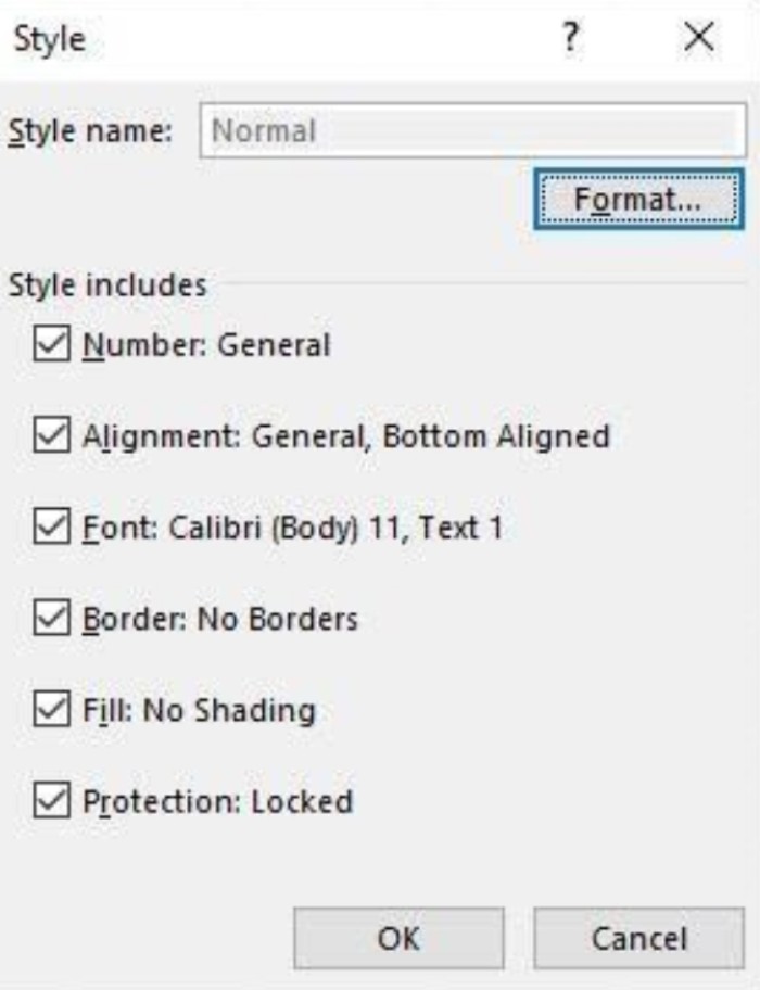
To quickly preview a style’s formatting without applying it, right-click the style in the gallery and choose “Modify.” The resulting dialog box (Figure B) displays the formats associated with the “Normal” style. Not all format types will be present, as it depends on the style.

Figure B

How to Efficiently Use Excel Styles

Working with Styles in Excel

If you are working with an existing workbook, chances are someone has already used one or more styles. Let’s take the example of opening Excel’s “Mortgage Calculator.xlsx” template. You will notice that the sheet contains data with formatting to enhance readability. Select a formatted cell and click the Cell Styles dropdown. In Figure C, you can see that cell I9 has the “Input” style applied, indicated by the heavy border around the current style in the gallery.

Figure C

How to Efficiently Use Excel Styles

It’s important to note that if you see formatting but the “Normal” style is selected in the Styles gallery, it means you are observing direct formatting, which was applied manually. Direct formatting is acceptable, but using it excessively alongside styles can lead to confusion. It’s better to modify the style rather than manually apply more formatting to a cell with an applied style.

Now, let’s see what happens when we modify the “Input” style for cell I9:

1. Click the Cell Styles dropdown and right-click on “Input.”
2. Select “Modify.”
3. In the resulting dialog box, click “Format.”
4. Go to the “Fill” tab and choose a different color, such as light orange.
5. Click “OK” twice.

As shown in Figure D, cell I9 now has a light orange background. Were you expecting all the gray cells in E3:E9 to change their fill color? (I was.) The explanation is simple: Only cell I9 is using the “Input” style. The gray cells in column E are using other styles, such

as “Amount,” “Percent,” and so on, which do not include a fill color. Therefore, the gray fill color in those cells is a result of direct formatting. Understanding the underlying styles helps you modify formatting with minimal confusion and effort. Remember, it is preferable to make changes to a style rather than relying on direct formatting.

Figure D

How to Efficiently Use Excel Styles

Now, let’s make a more significant change. Suppose you want to add bold formatting to the italicized cells in columns E and G and change the font color to dark green. You could use direct formatting on one of those cells and then use the Format Painter, but modifying the applied style is faster and ensures consistency in the future. Let’s try that:

1. Check one of the cells to see which style is applied (as I mentioned earlier).
2. Right-click the “Explanatory” style in the gallery.
3. In the resulting dialog box, click the “Format” tab.
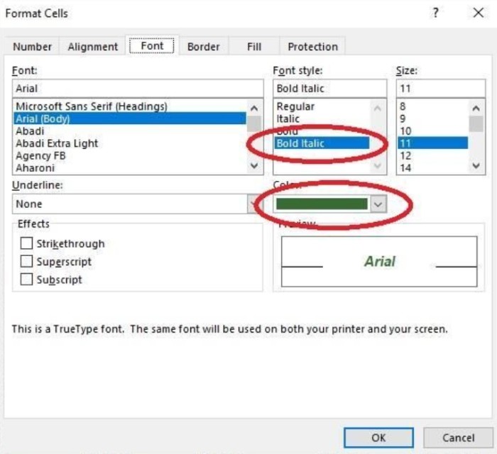
4. Go to the “Font” tab and change the Font Style to “Bold Italic.”
5. From the “Color” dropdown, choose dark green (Figure E).
6. Click “OK” twice.

Figure E

How to Efficiently Use Excel Styles

As shown in Figure F, the cells in columns E and G have been updated accordingly. It only took a few clicks to modify all those cells at once.

Figure F

How to Efficiently Use Excel Styles

By modifying the “Explanatory” style, we changed the formatting for several cells simultaneously. It’s important to remember that if you have other cells with the same style, they will also be updated. In most cases, this is desirable. However, if you want to preserve certain cells with their original formatting, you may need to create a new style. You can use the “Duplicate” option instead of modifying an existing style in the gallery, then assign a name to the new style and make the necessary changes. This approach is quicker than starting from scratch.

One Final Note

Cell styles in Excel are influenced by the theme applied to the entire workbook file. When you switch from one theme to another, cell styles will be adjusted accordingly.

Excel styles are easy to implement once you become familiar with them. Knowing that they exist, understanding which styles are applied, and how to modify them are key to using them efficiently. Embracing styles in Excel will help streamline your formatting processes and improve overall productivity.