How to search for data by row and column in Excel

Searching for data in Excel (finding values by row and column) is a common task for accountants. Typically, the VLOOKUP function is used to find data by column, and the HLOOKUP function is used to search by row to find the desired data. However, this method only applies when comparing item codes and corresponding values in a single search table. Therefore, if you need to find a value in both rows and columns, you should use a different method. In this article, Buffcom.net will guide you on how to combine the INDEX and MATCH functions to search for data by row and column.
Instructions for searching for data by row and column in Excel
1. INDEX and MATCH function structure
a. INDEX function structure
Syntax:=INDEX(reference; row_num; [column_num]; [area_num])
Where:
- reference: a required argument, is the reference area.
- row_num: a required argument, is the row number from which to return a reference.
- column_num: an optional argument, is the column number from which to return a reference.
- area_num: an optional argument, is the number of the range of cells to return the value within the reference.
b. MATCH function structure
Syntax:=MATCH(lookup_value;lookup_array;[match_type])
Where:
Lookup_value: is the value to be searched. It can be a number, text, or a reference cell.
Lookup_array: is the range of cells to search.
Match_type: determines the type of search. This parameter is optional. It can take one of the following values: 1, 0, -1. If you do not enter a value, Excel will default to a match type of 1.
- 1 or omitted: finds the largest value in the search range that is less than or equal to the lookup value. This type requires that the search range is sorted in ascending order, from smallest to largest or from A to Z.
- 0: finds the first value in the range that matches the lookup value exactly. This type does not require the search range to be sorted.
- -1: finds the smallest value in the range that is greater than or equal to the lookup value. The search range should be sorted in descending order, from largest to smallest or from Z to A.
2. How to combine the INDEX and MATCH functions to search for data
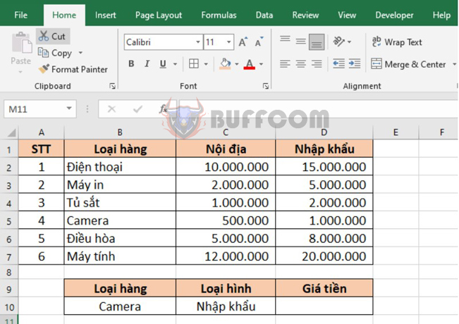
For example, we have a data table as shown in the image below. We need to reference the price of Imported Cameras in the table above.

How to search for data by row and column in Excel
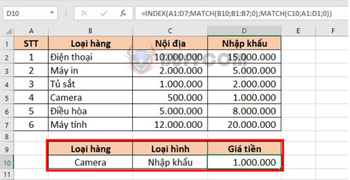
Applying the INDEX and MATCH function structure above, we have the formula to search for the price of Imported Cameras in the data table as follows:
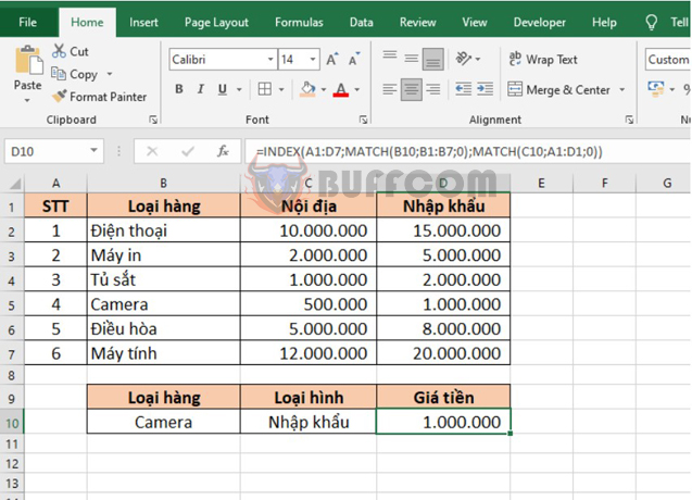
=INDEX(A1:D7;MATCH(B10;B1:B7;0);MATCH(C10;A1:D1;0))
The above formula means that we use 2 MATCH functions to return the column and row arguments of the INDEX function. Then the INDEX function will return the result which is the intersection of that column and row, which is the price of the imported camera that we are looking for.

How to search for data by row and column in Excel
Therefore, the article has instructed you how to combine INDEX and MATCH functions to search for data in Excel. Hopefully, this article will be helpful to you in your work. Wish you success!


