How to use the AVERAGEIFS function to calculate the average based on multiple criteria in Excel
How to use the AVERAGEIFS function to calculate the average based on multiple criteria in Excel: In Excel, the AVERAGEIFS function is used to calculate the average value of numbers in a range of cells that meet multiple conditions at the same time. You may wonder how AVERAGEIFS differs from AVERAGEIF. It’s simple: AVERAGEIF can only calculate the average value of cells that meet a single condition. If you have more than one condition, you need to combine it with another function or, more simply, use the AVERAGEIFS function. The following article will guide you on how to use the AVERAGEIFS function in Excel.
1, AVERAGEIFS function structure
Function syntax: =AVERAGEIFS(average_range; criteria_range1; criteria1; [criteria_range2; criteria2]; …)
Where:
- average_range: Required argument, the range to calculate the average value. It can include numbers, names, arrays, or references that contain numbers.
- criteria_range1, criteria_range2, …: criteria_range1 is a required argument, and the next criteria_range is an optional argument. These are the ranges of conditions.
- criteria1, criteria2, …: criteria1 is a required argument, and the next criteria are optional arguments. These are the conditions.
Note:
- If a cell in the criteria range is empty, the AVERAGEIFS function will default that cell to 0.
- If the average_range is empty or contains text, the AVERAGEIFS function will return the #DIV0! error value.
- Each criteria_range must have the same size and shape.
- If no cells meet all the criteria, AVERAGEIFS will return the #DIV/0! error value.
- Wildcard characters, question mark (?) and asterisk (*) can be used in conditions to substitute for characters.
2. How to use the AVERAGEIFS function
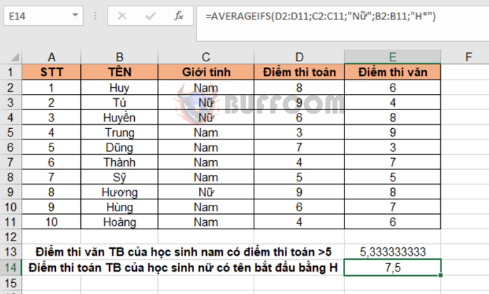
Let’s consider an example of a table showing math and literature scores of students as shown below.
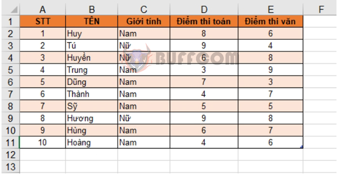
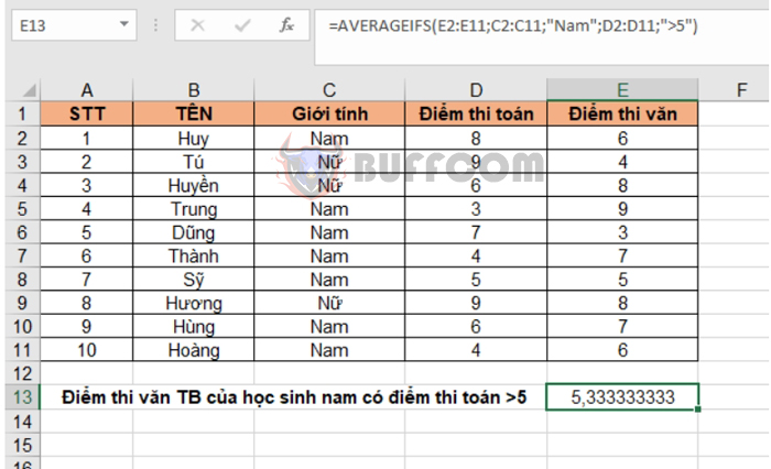
a. Calculate the average literature score of female students with math scores greater than 5.
=AVERAGEIFS(E2:E11;C2:C11;”Female”;D2:D11;”>5″)
Where:
- E2:E11 is the range of literature scores to calculate the average.
- C2:C11 is the range of gender conditions.
- “Female” is the condition for gender being female.
- D2:D11 is the range of math score conditions.
- “>5” is the condition for math scores greater than 5.
 b. Calculate the average math score of female students with names starting with “H”.
The formula would be: =AVERAGEIFS(D2:D11;C2:C11;”Female”;B2:B11;”H*”)
Where:
- D2:D11 is the range of math scores to calculate the average.
- C2:C11 is the range of gender conditions.
- “Female” is the condition for gender being female.
- B2:B11 is the range of name conditions.
- “H*” is the condition for names starting with “H”. The asterisk (*) is used as a wildcard for characters.
How to use the AVERAGEIFS function to calculate the average based on multiple criteria in Excel
That’s it! The above article has guided you on how to use the AVERAGEIFS function in Excel. Good luck!

