How to Use VLOOKUP and MATCH Combination in Excel

The combination of VLOOKUP and MATCH functions in Excel is like having a superpower. VLOOKUP is one of the most commonly used functions in Excel, which helps to lookup a value in a column quickly. However, the biggest issue with VLOOKUP is that it is not dynamic, as col_index_num is a static value. This means that when working with multiple-column data, it is a hassle to change the reference manually.
To address this issue, the MATCH function can be used in VLOOKUP for col_index_number. This post will explain how to use this combo formula effectively.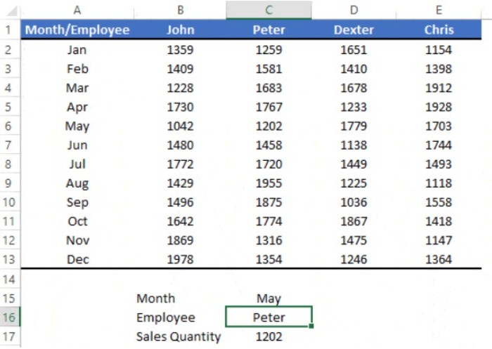
Problems with VLOOKUP
There are two major reasons why the combination of VLOOKUP and MATCH is needed. The first issue is the static reference. For instance, if you have a table of 12-month sales for four employees and you want to look up the sales for a specific month and employee, you need to specify the column number manually.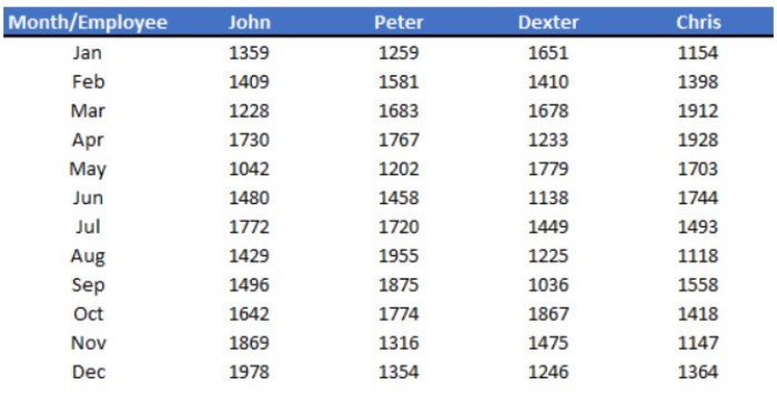 This means that if you need to change the employee or add/delete columns, you need to change the col_index_num manually.
The second issue is adding or deleting columns. If a new column is added, the col_index_num value needs to be adjusted manually.
Why Use the MATCH Function?
Before combining VLOOKUP and MATCH, it is essential to understand how the MATCH function works. The MATCH function returns the cell number of the lookup value from a range. 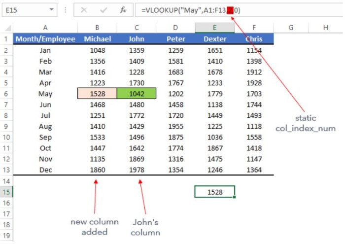 It has three main arguments: the lookup value, a range to lookup for the value, and the match type to specify an exact match or an approximate match.
Combining VLOOKUP and MATCH
To combine VLOOKUP and MATCH, the following steps can be followed:
- Enter the month’s name and the employee’s name in separate cells.
- In a third cell, enter the formula =VLOOKUP(C15,A1:E13,MATCH(C16,A1:E1,0),0).
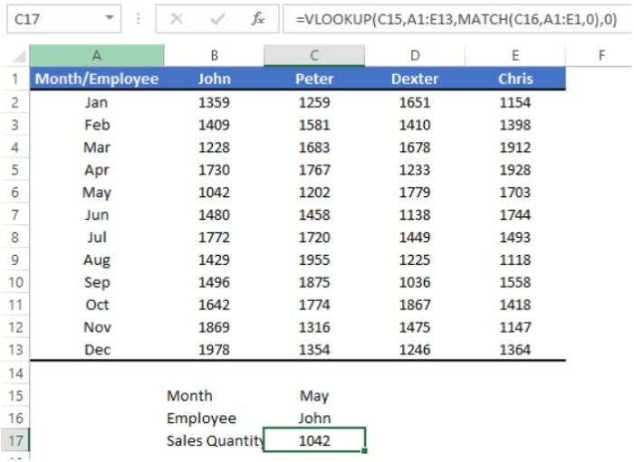
- The MATCH function in the formula will return the column number for the employee’s name.
- The VLOOKUP function will then use the returned column number to find the corresponding value in the specified row.
- The 0 at the end of the formula signifies that an exact match is required.
In summary, combining VLOOKUP and MATCH functions can make Excel more dynamic and efficient when working with large datasets.
The formula above uses VLOOKUP to search for data in the MAY month, and instead of a static value for the col_index_num argument, it uses the MATCH function. The MATCH function looks up the employee name “John” to find the column number for VLOOKUP to retrieve the value.
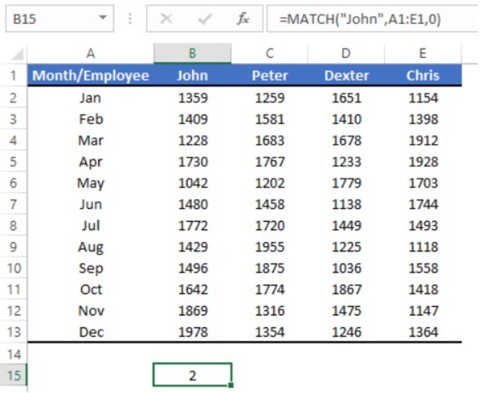
Essentially, the MATCH function provides the correct column number for VLOOKUP to retrieve the value. This solves two problems caused by using a static col_index_num value.
Firstly, by using the employee name in the MATCH function to obtain the column number for VLOOKUP, the col_index_num value becomes dynamic. When you change the employee name in the cell, the MATCH function changes the column number accordingly. This means you no longer need to edit the formula repeatedly when getting data for different employees.
Secondly, when a new column is added or deleted, the MATCH function updates its value to reflect the correct column number for the employee’s data.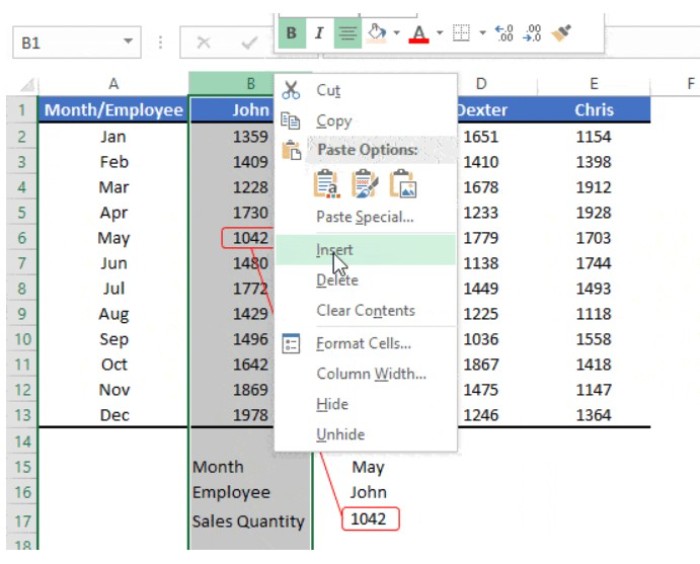 This ensures that the formula continues to provide the correct data even when columns are added or deleted.
Therefore, by combining VLOOKUP and MATCH, you can always get the correct column number for retrieving data using VLOOKUP, even if columns are added or deleted.


