How to utilize Excel’s Find feature for highlighting or deleting matching values

How to utilize Excel‘s Find feature for highlighting or deleting matching values. When working with large workbooks or sheets containing numerous columns and rows, the ability to quickly find specific values is essential. In addition to understanding the basic functionality of the Find feature, you can leverage it even further by formatting or deleting matching values.

Basics of Find feature

You are likely familiar with Excel’s Find feature, which allows you to search for specific values. However, you may not have explored its capabilities beyond simple search tasks. The basics are straightforward.

Before initiating a search, you need to decide whether to search the entire workbook or a specific range. If you want to search within a range, select it first. To search the entire workbook, click on any cell in the active sheet. Searching within a specific range is more efficient and is recommended whenever applicable.

To access the Find feature, press Ctrl+F to open the Find and Replace dialog. Alternatively, go to the Editing group on the Home tab and click on Find & Select, then choose either Find or Replace from the dropdown menu. Both options are available within the same dialog.

Options for Find

I recently encountered a situation where an Excel application heavily relied on simple find tasks but stopped working, leaving users perplexed. Upon investigation, it turned out that an option had been inadvertently changed, causing Excel to search for values within formulas instead of searching for values directly. Even though the file didn’t contain any formulas and was a straightforward data-tracking sheet, the search results were unexpected and erroneous. The issue lied with the option settings rather than Excel itself.

How to utilize Excel’s Find feature for highlighting or deleting matching values

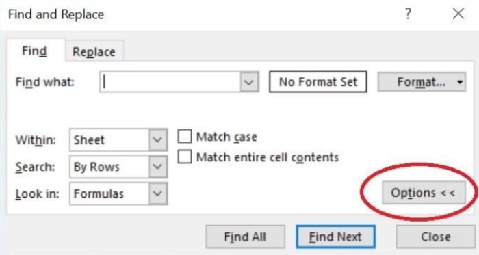
To access the options, as shown in Figure A, click on the Options button within the Find and Replace dialog. These options allow you to fine-tune your search:

• Within: Determines the scope of the search, either within the active sheet or the entire workbook. The default is set to the active sheet, but you can change it to search the entire workbook.
• Search: Specifies the search direction, either by columns or by rows. Although changing this option isn’t crucial, it can potentially speed up the search. The default setting is By Rows.
• Look in: Allows you to limit the search to formulas, values, or comments. Selecting the wrong option can lead to undesired results, as mentioned earlier. The default setting is Formulas, strangely enough. Use the Formulas option to quickly update references.
• Match case: Finds only those values that match the case (uppercase or lowercase) specified in the Find what field. The default setting is disabled.
• Match entire cell contents: Finds only those values that exactly match the characters entered in the Find what field. This option is useful for locating exact or similar matches based on your settings. The default setting is disabled.
• Format: Enables searching for specific formats, which is particularly useful if you don’t rely heavily on cell styles. You can use the Replace feature to update formats through a simple search task. The default setting is disabled.

Figure A showcases the Find options within the dialog.

Using the appropriate options is key to executing efficient search tasks. Excel’s Find and Replace feature remembers your previous settings, which can lead to unexpected issues. Unfortunately, there isn’t a straightforward option to reset everything, so you must remember to check the options each time you perform a search to avoid inaccurate results.

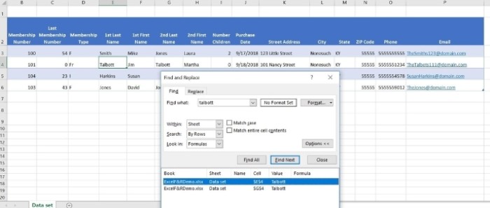
While the basics are easy to grasp, it’s equally important to understand what actions you can take with the search results. You can view, select, highlight, and even delete matching values. Figure B illustrates the outcome of initiating the Find and Replace dialog, entering “Talbott” as the search term, and clicking on Find All. The dialog returns a list of every instance of the search term based on the specified options. In this example, all the default options were used. Let’s examine the results within this context.

How to utilize Excel’s Find feature for highlighting or deleting matching values

Figure B:

A search term may not always find the expected values.

The search results display both instances of “Talbott” in row 4. Even if one instance used a lowercase “t” (as in “talbott”), the list would remain the same. However, it’s important to note that the search doesn’t find the email address because the search term is not spelled the same way (“Talbots” instead of “Talbott”). The absence of the second “t” prevents the match. If either of the name fields had a missing “t,” Excel would not find it either.

To access one of the found items, double-click it in the list. If you click “Find Next,” Excel will move to the next cell containing the search term instead of displaying a list in the dialog.

Highlighting or deleting matching results:

While the aforementioned features may be sufficient for most users, there are additional actions you can perform. For instance, using the search task, you can highlight or even delete matching entries. To demonstrate this, let’s repeat the same search task and then proceed with highlighting and deleting those values (note that I added the second “t” to the email address).

1. Click on any cell in the active worksheet and press Ctrl+F to open the Find and Replace dialog.
2. In the “Find What” field, enter “Talbott” (including both “t”s).
3. Click on “Options” if necessary and ensure that all the options are set to their defaults.
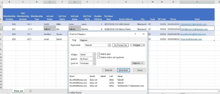
4. Click on “Find All” to display the list shown in Figure C.
   

   How to utilize Excel’s Find feature for highlighting or deleting matching values

   Observe that the first matching item in the list is automatically selected. Do not make any changes at this point!

5. While the selection is active in the resulting list, press Ctrl+A to select all matched items. Excel will also highlight the cells at the cell level (although it may be difficult to distinguish in the case of the email address, as it is the last matching value and therefore the active cell, resulting in a different appearance for the selection).
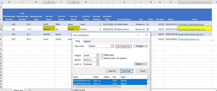
6. Once you have selected all matching cells, you can highlight them by choosing a fill color option from the Font group on the Home tab (see Figure D). At this stage, you can apply other formats as desired.
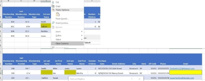
7. Alternatively, right-click on any cell within the selected group of cells and choose “Clear Contents” (see Figure E). However, exercise caution when performing this action. Remember that you can press Ctrl+Z to undo any changes if needed. (Pressing the Delete key on the keyboard will delete the list in the dialog, not the matching entries at the sheet level.)

Figure C:

Displaying all matches.

Figure D:

How to utilize Excel’s Find feature for highlighting or deleting matching values

Using a fill color to highlight the matching entries.

How to utilize Excel’s Find feature for highlighting or deleting matching values

Figure E:

Deleting the entries.

Stay tuned:

Even if you are already familiar with the basic purpose of this feature, you have now learned how to expand its functionality by applying formats or deleting matching values. In the following month, we will explore more advanced techniques.

Feel free to send me any questions you have regarding Office. While I try to answer reader questions when possible, please note that there is no guarantee. Unless requested, please avoid sending attached files with your initial help requests, as such messages will be deleted without being read. If necessary, you can provide screenshots of your data to clarify your question.