How to Refresh Data Connections and Pivot Tables using Excel VBA

How to Refresh Data Connections and Pivot Tables using Excel VBA. This article will guide you through creating multiple PivotTables and refreshing all data connections and PivotTables using VBA in Excel.

How to Refresh Data Connections and Pivot Tables using Excel VBA

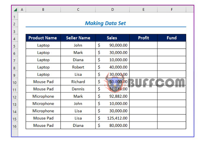
Step 1: Create a Data Set

First, create a data set including Sales, Profit, Fund, Product Name, and Seller Name (as shown below) to identify errors.

How to Refresh Data Connections and Pivot Tables using Excel VBA

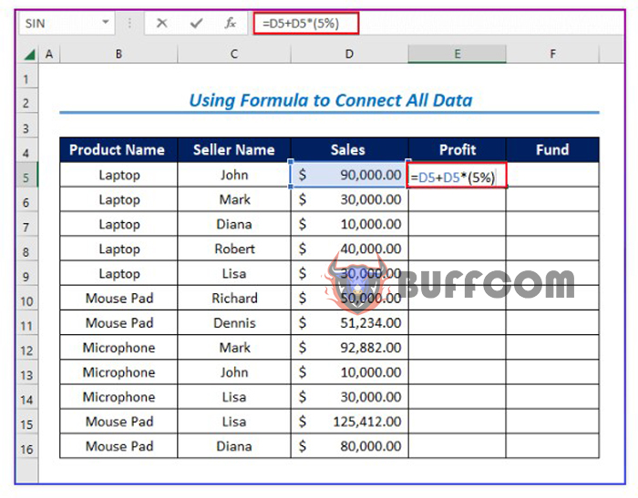
Step 2: Link Data Using Formulas

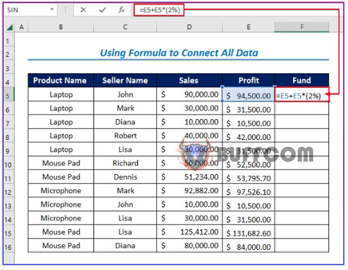
Calculate Profit and Funds by entering formulas as shown below.

How to Refresh Data Connections and Pivot Tables using Excel VBA

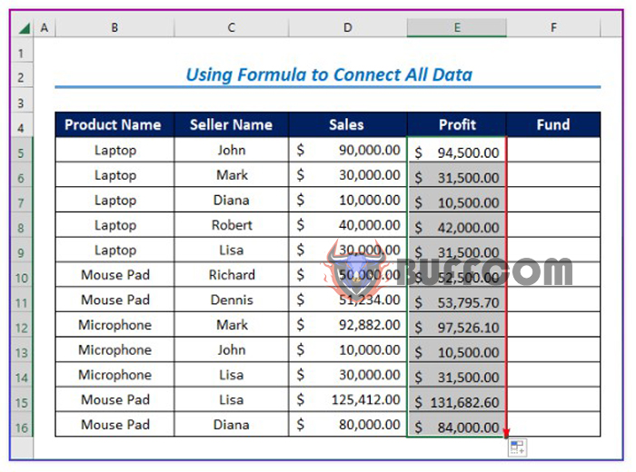
Then, press Enter to display the results.

How to Refresh Data Connections and Pivot Tables using Excel VBA

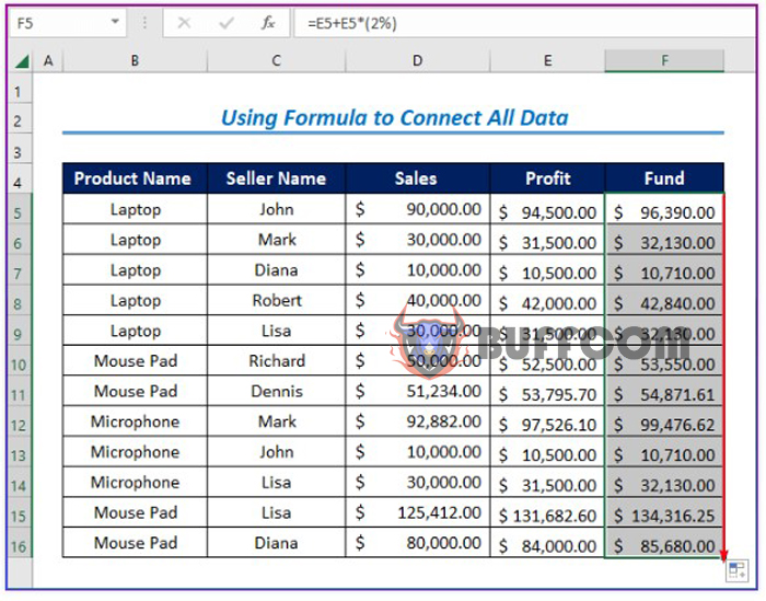
Similarly, calculate Funds using the formula shown below.

How to Refresh Data Connections and Pivot Tables using Excel VBA

The results will be displayed.

How to Refresh Data Connections and Pivot Tables using Excel VBA

Step 3: Create a PivotTable from the Data Set

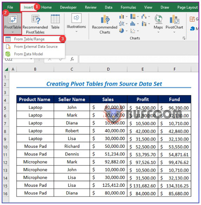
Create a PivotTable by selecting Insert > PivotTable

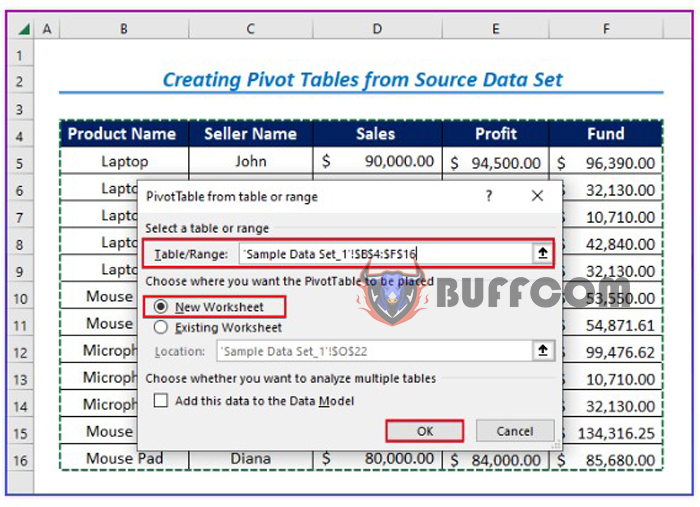
Then selecting From Table/Range, and choosing the data range.

Select New Worksheet, then click OK.

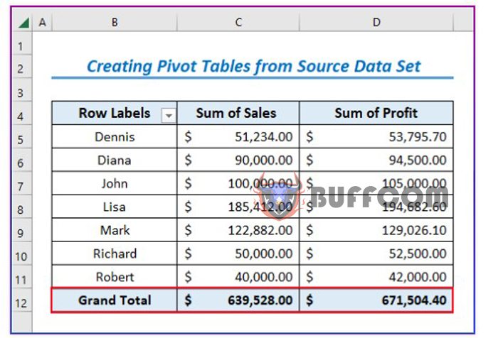
Finally, the PivotTable will display the total Sales, Funds, and Profits (as shown below).

Step 4: Change Values in the Source Data Set

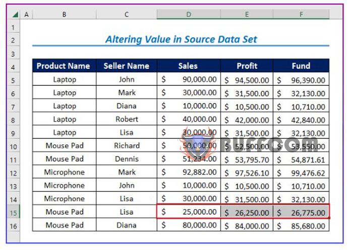
Change the value by entering 25000 in cell D15. Then, you can see the changes in the corresponding values in cells E15 and F15.

Step 5: Enter VBA Code to Refresh Data in the PivotTable

Select Developer > Visual Basic

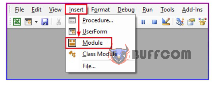
Then select Insert > Module.

Enter the following code:

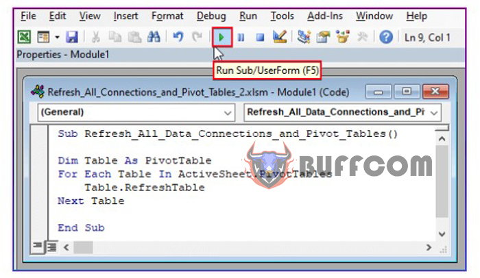Sub Refresh_All_Data_Connections_and_Pivot_Tables()
Dim Table As PivotTable
For Each Table In ActiveSheet.PivotTables
Table.RefreshTable
Next Table
End Sub

Press F5 to run the code.

Step 6: Display the Final Result with Refreshed Values in the PivotTable

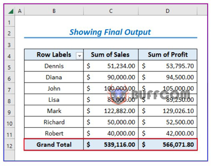After refreshing the data, you will see that all data is automatically refreshed in the PivotTable.