Tips for Numbering Rows and Columns in Excel for Office Workers

When we talk about Excel, we often think of formulas, complex calculations, and scripts that help us work quickly. In this article, Buffcom.net will summarize ways to number rows and columns in Excel.

Aside from its ability to create tables or perform complex calculations, Excel also has many small but extremely useful features. For example, if you have a long list of human resource management, employee lists, or phone numbers, you can easily number the rows you need to manage with just one click of a mouse in Excel, without having to click on each cell and enter each number. This can be inconvenient, unprofessional, and sometimes lead to errors in a particular location if the table contains hundreds or thousands of numbers that need to be entered.

If you don’t know how to number rows and columns in Excel, this is an article for you. The Excel application is a programming editor and text statistics tool, so it is also integrated with many useful tools and features to make your statistical and calculation work more convenient, faster, and more accurate. Below is a detailed guide:

I. Four Ways to Number Rows and Columns in Excel 2007, 2010, 2013, 2016

Method 1: Number directly into each cell in Excel, this is the most manual and easy-to-use method when the number of rows and columns is not too large. For row numbers greater than 30, this will be a big obstacle to your statistical work.

Method 2: Number rows and columns in Excel by dragging the mouse. With just two steps:

Step 1: Enter the first two row numbers.

Step 2: Highlight the two cells just filled with numbers, then place the cursor at the corner of the cell until the cursor changes to a plus sign, and begin dragging down to the desired row number.

Method 3: Number rows and columns in Excel with a formula. With just two steps:

Step 1: Enter the first row number.

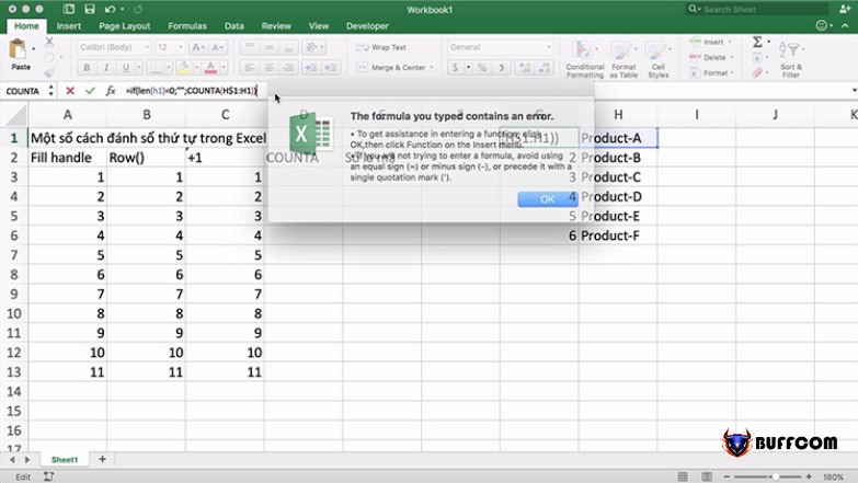
Step 2: Enter the formula =cell position just filled with number + n (depending on how you want to number rows, continuously n=1, odd numbers n=2, etc.).

Method 4: Number rows and columns in Excel with the Fill tool.

II. Instructions on how to auto number in Excel

1. Use the Fill Series feature to quickly number sequentially

Step 1: Open the Excel file that you want to number sequentially. For example, I have an Excel file.
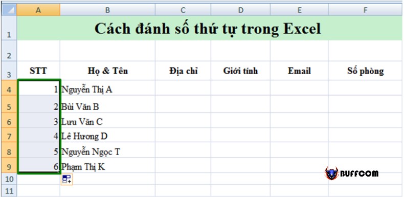
Step 2: Enter the number 1 into the cells where you want to start the numbering. Click on that cell => then move the cursor to the bottom right corner of that cell => a plus sign will appear like the image below => left-click and drag down to the position where you want to end.
Step 3: At this point, an icon with a feature will appear next to it. Click on that triangle icon as shown below => then check the Fill Series option to create sequential numbers along the rows as you want. And this is the result.

2. Auto-number in Excel using the Ctrl key (recommended)

Open the Excel file => then enter the number 1 into each cell where you want to start numbering.

Left-click on the cell where you just entered the number => move the cursor down to the bottom right corner of the cell you just selected => a plus sign will appear like the image below => now hold down the Ctrl key while dragging the cursor down to the position where you want to end.

Do the same as method 1 but with an additional step of holding down the Ctrl key. This is an important formula for auto-numbering in Excel.

III. How to write a 0 in front of a number in Excel

1. Enter a single quote before the number sequence you want to enter.

Excel will automatically remove that quote, but there will be a warning triangle above it.

2. Select the column format as Text.

Step 1: Select the column to create a 0 in front of the number => right-click => select Format Cells
Step 2: The Format Cells dialog box will appear. In the Category section, select Text => OK
The result is that when you enter a 0 at the beginning of the sequence, it will not disappear.

3. Use Custom

Step 1: Select the column you want to write the 0 in front of the number => right-click => Format Cells
Step 2: The dialog box appears, select Custom => In the Type section, enter the number of 0 digits you want to display (assuming you choose 12) => OK.

IV. Some other types of numbering in Excel that you may be interested in

1. How to repeat sequence numbers in Excel

Step 1: First, you should name both sheets: one for the list of each student and one for the exam room, instead of using the default names. You can also name them as you like.
Step 2: In the sheet for the exam room, select the data range, leaving only the column name, and then go to Formulas > Defined Names > Define Name. Here, we will assign the name “V” to this data.
Step 3: Go back to the sheet of the list of students and input the sub-number for the first student as 1. Then, enter the following formula for the second student: =IF(B3=5,1,B3+1).
Step 4: Then, copy all the columns below to see the results of repeating sequence numbers in the formula for numbering in Excel.
Step 5: Next, in the exam room cell, column F, enter the following formula: =IF(A3=5,”V”,VLOOKUP($A$3,A,2)).

This is a conditional function that also searches for data. If the cells meet the conditions of the data “V” in the Sheet, the corresponding result with Column B in the exam room sheet will be displayed.

Step 6: The result will be as shown below. Simply copy it to most of the columns below, and the formula for numbering in Excel will be completed with repeated sequence numbers.
The final result of numbering with repeated sequence numbers in the formula for numbering in Excel will be as shown below. Of course, this example only applies to lists of 10 people, but imagine if we use sequence numbers that repeat in one or a few cycles in the formula for numbering in Excel with lists of up to 1000 people, the efficiency of this trick will be clear. If you have any questions or encounter any problems during the process, please leave a message here. The management team will help you clarify any concerns.

2. Numbering pages between sheets in Excel in order

Step 1: First, name both sheets: one for the list of each student and one for the exam room, instead of using the default names. You can also name them as you like.
Step 2: In the sheet for the exam room, select the data range, leaving only the column name, and then go to Formulas > Defined Names > Define Name. Here, we will assign the name “V” to this data.
Step 3: Go back to the sheet of the list of students and input the sub-number for the first student as 1. Then, enter the following formula for the second student: =IF(B3=5,1,B3+1).
Step 4: Then, copy all the columns below to see the results of repeating sequence numbers in the formula for numbering in Excel.
Step 5: Next, in the exam room cell F column, we will enter the following formula: =IF(A3=5,”V”,VLOOKUP($A$3,A,2)). This is a conditional function combined with data lookup. If the cell satisfies the data condition, “V” will be outputted in the corresponding result column B in the exam room sheet.
Step 6: The results will appear. Here, we just need to copy the column below, and the sequential numbering in Excel will be completed in cycles.

3. Error in numbering in Excel

Step 1: Instead of just typing 1, you need to type both 1 and 2. You can also type the numbers sequentially as 1, 2, 3, and so on.

Step 2: Then, highlight both 1 and 2, and click on the corner of 2 so that the cursor becomes a plus sign (+). Then, click and drag the mouse downwards.

Step 3: Immediately afterwards, you will get a series of sequential numbers as desired. If you want to extend the sequential numbers, highlight all of them and continue with the drag and drop operation.

And you can easily fix errors in Excel sequential numbering by just adding the missing number 2 as a “seed” for Excel to understand your intention of carrying out a series of sequential numbers.

In addition to this method of numbering in Excel, there is another important trick related to ordering. That is creating the Rank function in Excel.

V. How to sort data in Excel (accurate way)

1. Simple sorting in Excel

What is the numbering of rows in Excel? Sorting can be very simple, with a process of just 2 clicks to help you sort the data in your spreadsheet. Let’s learn how to do it together.

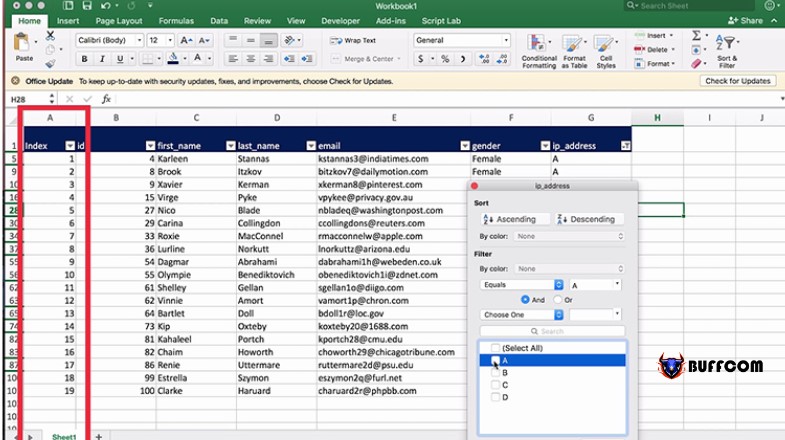
In the exercise of numbering rows in Excel, start by clicking on a row of the column you want to sort. Now, make sure you are on the Home tab in the ribbon bar, and find the Sort and Filter button located far to the right of that bar.

Note that with these sorting options, you can sort the data in “A to Z” or “Z to A” order. These simple options will sort data in Excel 2007 in alphabetical order, and in which direction depending on the option you choose.

Once you have sorted the data in numbering rows in Excel, all the rows will be sorted accordingly. Basically, the column you selected will be the “key” that Excel uses to determine how to sort that data. But each row is a record, so they need to be grouped together.

It’s really easy to perform this basic sorting. Simply click on the data column, then choose a sorting method, and Excel will sort the data in that spreadsheet in order.

2. How to avoid sorting your Excel data.

The issue that arises is when you have a large data spreadsheet, but you accidentally sorted only one column of data. Each of those data rows in Microsoft Excel will look like a copy of the previous one, through the rows.

The biggest mistake every Excel user encounters is only selecting one single column when sorting, and selecting incorrectly in the next window.

The numbering options in Excel will warn us, with a window labeled Sort Warning. That pop-up window will have choices for expanding the selection (choose this) or continuing with the current selection.

I always think the choices in this window can be difficult to understand fully. Just know that you will want to use Expand the selection to ensure that the numbering options in Excel will include all columns when sorting data.

For testing purposes, we will see what happens when we select one column and choose the sorting sample Continue with the current selection.

Do not use the option Continue with current selection if you are working with a single column – make sure to expand your data selection.

3. Advanced Excel Sorting

How can we know about Excel numbering:

Sorting alphabetically by table, then by country in a spreadsheet.

Sort by the alphabetically by customer name, then by the type of job we did for them.

Sort the part of the customers in a list alphabetically, then by the amount of each individual project, from largest to smallest.

The answer to all of these is advanced sorting, where you can set multiple levels of sorting when sorting data. We’ll dive into the last example using a data template.

To start, click anywhere within your data and find the Sort & Filter option, then select Custom Sort.

In my case, I will select Client from the drop-down menu, set Sort On to Values, and set Order to A to Z. This will sort the Excel numbering according to the spreadsheet and based on alphabetical order.

When you click OK, the Excel numbering will sort the spreadsheet based on the rules you have set in this window.

4. Summary and further learning.

Sorting is an essential skill that spreadsheet users need to have to be prepared for their Excel numbering operations. When you need to reuse old data in your spreadsheet, it can take too much time to cut and paste in a specific order. Therefore, sorting is necessary.

You can always develop the skills you have learned today by referring to other excellent tutorials on how to number in Excel.

Learn how to work with Excel formulas at How to manage your formulas in Excel numbering.

VI. Excel does not calculate formulas

1. You have entered a formula in a cell formatted as Text.

In the image above, we can see that cell B5 is formatted as Text, so the formula cannot be automatically calculated. The solution is to change the format of cell B5 to General, Number, or any other format except Text. Then, enter the formula again or press F2 and Enter.

2. Excel is in formula display mode

This is one of the options for displaying cell contents in Excel, which can be set under Options/ Advanced/ Show formulas in cells instead of their calculated results (or by using the shortcut key Ctrl + `).

In this mode, all the formulas on a sheet will only display the contents of the formula without showing the result.

To fix this:

Turn off this feature by unchecking Show formulas in cells instead of their calculated results.
Or you can press Ctrl + ` again to turn off the display of formulas only.

Why does Excel have a formula display mode?

To help users edit formula content faster, the formula display mode in Excel allows the sheet to be displayed in a way that only shows the formula, making it easier and faster to edit the formula content without confusing it with other contents.

3. You are in manual calculation mode in Excel

As shown in the image above, the Workbook calculation is set to Manual. You need to change it to Automatic in order for Excel to automatically calculate the formula in the numbering method. Here’s how:

For Excel 2010, go to Tools > Options… > Options window appears > Select the Calculation tab > Check Automatic > Press OK to save settings, and now you can view the result!

For Excel 2010 and later versions, go to File > Options > Select Formulas in the left column > Check Automatic on the right side > Press OK.

Alternatively, you can press F9 to recalculate the formula each time you want to calculate the numbering method in Excel. With these methods, you will need to press F9 each time you want Excel to recalculate.

4. Your formula is experiencing Circular References

In this case, the formula will always result in zero. The solution is to identify and remove the circular reference.

To check for circular references, follow the steps in the image above: Under the Formulas tab, select Error Checking, and then select Circular References. The numbering system in Excel will guide you to the cells that contain circular references (cells that are cross-referenced multiple times). Review the formulas that are cross-referenced, and adjust or paste the value of one of them. Two formulas cannot directly or indirectly add to each other through a third cell. Therefore, you must adjust or paste the value of one formula in order to calculate the final formula.

VII. Conclusion
So, we have just shared with you an entirely automated method to number rows in Excel. Although this is a small trick in Excel, it is extremely useful in many cases when working with row numbering in Excel. If you work with Excel, it is essential and necessary to apply this feature to your work if you want to be successful with row numbering in Excel. We hope that this sharing will be useful to you in both your studies and work. Good luck!