How to use Vlookup and Hlookup that few people know in Excel

Vlookup and Hlookup are two very popular functions used in Excel. Despite their widespread use, many people may not fully utilize the potential of these common functions. In today’s article, let’s explore the lesser-known uses of Vlookup and Hlookup through small examples.
Hlookup function
For the less known usage of Vlookup and Hlookup functions, let’s take an example of a clothing store. After obtaining the customer’s waist measurement, we need to find the corresponding size from the size chart available. First, we need to extract the waist measurement value from the size chart. Note that, for example, 63-66 means the waist measurement is greater than 63 and less than or equal to 66. To obtain the first number, we use the LEFT function with the first parameter being the cell containing the value and the second parameter being 2 (because the waist measurement in the table consists of only 2 digits). In cases where the measurement is less than 63 or greater than 90, you need to enter the value manually.
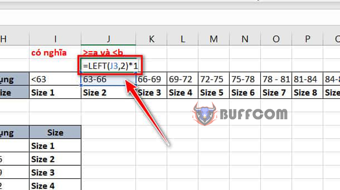
How to use Vlookup and Hlookup that few people know in Excel
After completing the above operation, next, we will use the Hlookup function. This function will include 4 arguments: the cell containing the waist measurement value, our size chart (consisting of 3 rows, including the row with the first measurement value we just created above. Note to press F4 once to fix this table), the row number containing the value to be returned, and finally, the value TRUE or 1. Once completed, you can drag the formula down to apply it to the cells below.
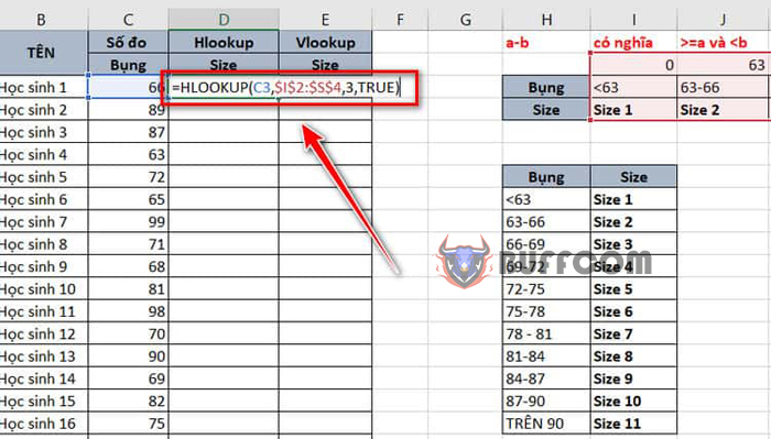
How to use Vlookup and Hlookup that few people know in Excel
Vlookup function
With the Vlookup function, we will also perform a similar process as with the Hlookup function. First, we need to obtain the waist measurement value in the size table. You will also use the LEFT function with 2 parameters like the Hlookup function, including the cell containing the measurement value and the number 2. The only difference is that our size table will be represented in columns instead of rows as above. For cases smaller than 63 or larger than 90, you need to manually enter them.
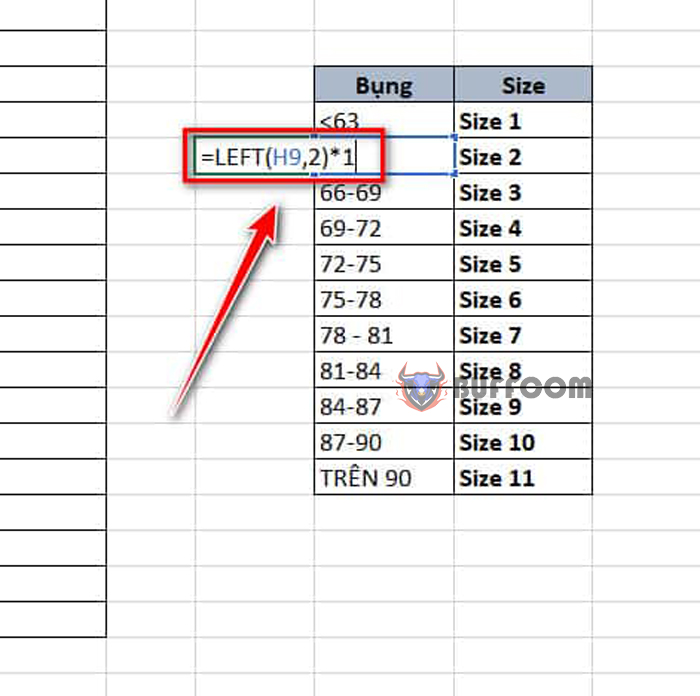
How to use Vlookup and Hlookup that few people know in Excel
Next, we will use the Vlookup function to get the size number from the given waist measurement value. The Vlookup function takes 4 parameters including: the cell containing the measured waist size, the size table (including 3 columns, including the row with the first measurement value just created. You should also remember to press F4 once to fix the size table), the column number containing the returned value, and finally the TRUE or 1 value. Once done, you can drag from the first cell down to apply to the cells below. Good luck with your practice!
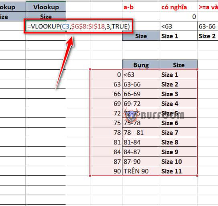
How to use Vlookup and Hlookup that few people know in Excel
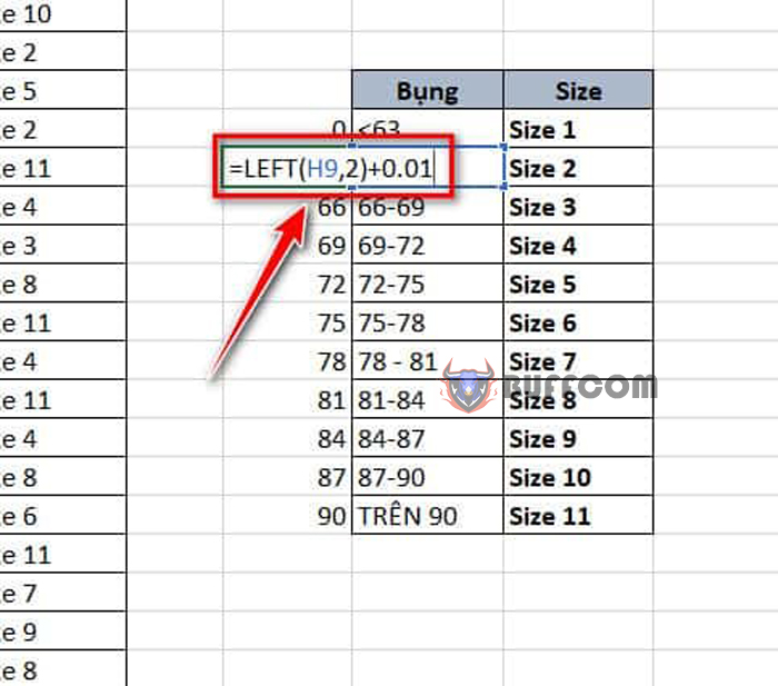
How to use Vlookup and Hlookup that few people know in Excel
In the case of the size table being 63-66 and your condition being greater than or equal to 63 and less than 66 instead of greater than 63 and less than or equal to 66 as in the example above. When obtaining the waist measurement value in the table, after the LEFT function, you add a very small number (for example, 0.01) instead of multiplying by 1. At this time, in the data table, a student with a waist measurement value of 63 will become size 1, while before the modification, it would have been size 2.
In conclusion, learning how to use Excel functions such as HLOOKUP and VLOOKUP can greatly improve your productivity and efficiency in data analysis and management tasks. By following the step-by-step instructions and tips provided, you can confidently apply these functions to your own Excel projects. Remember to always practice and explore different ways to use Excel functions to optimize your work process.


