Using the TRIM Function in Microsoft Excel 2010
Using the TRIM Function in Microsoft Excel 2010. In this article, we will explore how to remove unnecessary blank characters from a cell using the “TRIM” function in Microsoft Excel 2010.
The TRIM function is employed to eliminate any extra leading and trailing spaces from the text within a cell.
Using the TRIM Function in Microsoft Excel 2010
The syntax of the TRIM function is as follows: =TRIM(text).
For example, let’s say Cell A2 contains the text “Excel Tips”. To remove the unnecessary spaces, you can enter the formula “=TRIM(A2)” in Cell B2 and press Enter on your keyboard. The function will return the text without the additional spaces.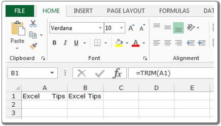
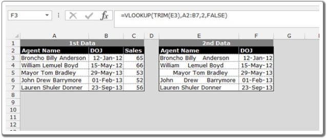
Now, let’s consider a practical example to understand where and how we can use the TRIM function. Suppose we have two datasets: the first dataset contains all the details, and we want to extract the date of joining for each employee in the second dataset using their names.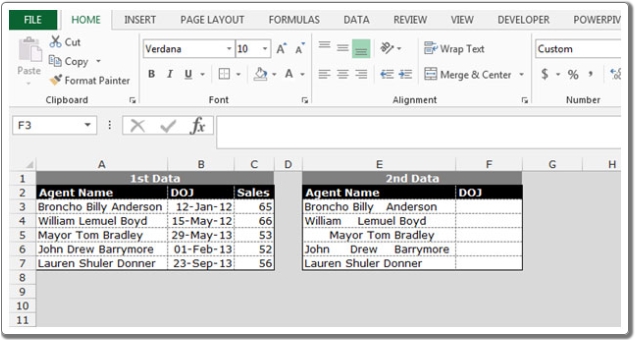
Since the employee names may have spaces, we can utilize the TRIM function in conjunction with the VLOOKUP function. Follow the steps below:
- Write the formula in Cell F2: =VLOOKUP(TRIM(E3), A2:B7, 2, FALSE).
- Press Enter on your keyboard.
- The function will return the date of joining for the corresponding employee.
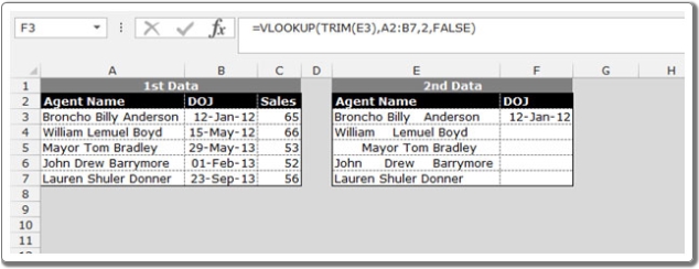
To apply the formula to the remaining cells, copy the formula by pressing Ctrl+C and paste it into the range F3:F7 by pressing Ctrl+V on your keyboard.
By using the TRIM function alongside other functions like VLOOKUP, you can effectively manipulate and extract data from cells in Microsoft Excel 2010.