Steps to create a summary table of customer accounts receivable in Excel

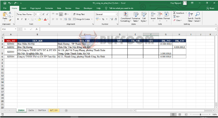
Step 1: DMKH Sheet

Here, you enter basic information about customers such as code, name, address, tax code, bank account, phone number, beginning balance, and beginning credit balance.

Steps to create a summary table of customer accounts receivable in Excel

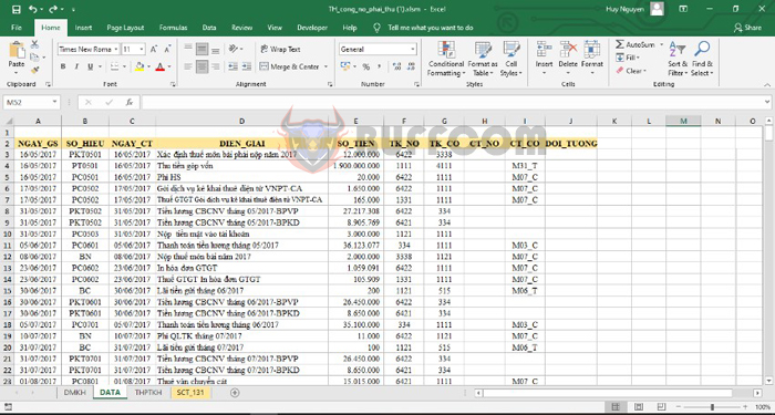
Step 2: DATA Sheet

Here, you enter the transactions that occur during the period. The information you need to enter includes the date, reference number, description, amount, debit account, credit account, and customer.

Steps to create a summary table of customer accounts receivable in Excel

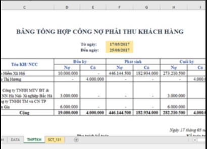
Step 3: THPTKH Sheet

Here, you will summarize data from the DMKH sheet to obtain the beginning balance, and retrieve data from the DATA sheet to obtain the transactions occurred during the period. Then, add the beginning balance and the transactions to get the ending balance.

• In the Debit opening balance column, enter the following formula:
  =MAX(VLOOKUP(B11, DMKH!$A$3:$H$6, 7, 0) – VLOOKUP(B11, DMKH!$A$3:$H$6, 8, 0) + SUMIFS(SO_TIEN, CT_NO, B11, NGAY_GS, “<” & $F$6) – SUMIFS(SO_TIEN, CT_CO, B11, NGAY_GS, “<” & $F$6), 0)
• In the Credit opening balance column, enter the following formula:
  =-MIN(VLOOKUP(B11, DMKH!$A$3:$H$6, 7, 0) – VLOOKUP(B11, DMKH!$A$3:$H$6, 8, 0) + SUMIFS(SO_TIEN, CT_NO, B11, NGAY_GS, “<” & $F$6) – SUMIFS(SO_TIEN, CT_CO, B11, NGAY_GS, “<” & $F$6), 0)
• In the Debit transactions column, enter the following formula:
  =SUMIFS(SO_TIEN, CT_NO, B11, NGAY_GS, “>=” & $F$6, NGAY_GS, “<=” & $F$7)
• In the Credit transactions column, enter the following formula:
  =SUMIFS(SO_TIEN, CT_CO, B11, NGAY_GS, “>=” & $F$6, NGAY_GS, “<=” & $F$7)
• In the Debit closing balance column, enter the following formula:
  =MAX(D11 + F11 – E11 – G11, 0)
• In the Credit closing balance column, enter the following formula:
  =-MIN(D11 + F11 – E11 – G11, 0)

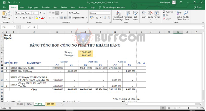
Steps to create a summary table of customer accounts receivable in Excel

Step 4: Sheet SCT_131

Here, we will create a detailed ledger for each object. We will consolidate data from the DMKH sheet to obtain the beginning balance and data from the DATA sheet to obtain the incurred debit and credit amounts for the period. Then, we will add the beginning balance and the amounts incurred during the period to obtain the ending balance of the object.

• In the Beginning Debit column, you will enter the following formula:
  =MAX(VLOOKUP(G10;DMKH!A3:H6;7;0) + SUMIFS(DATA!E3:E251;DATA!A3:A251;”<“&G8;DATA!H3:H251;G10)-
  VLOOKUP(G10;DMKH!A3:H6;8;0) – SUMIFS(DATA!E3:E251;DATA!A3:A251;”<“&G8;DATA!G3:G251;G10);0)
• In the Beginning Credit column, you will enter the following formula:
  =-MIN(VLOOKUP(G10;DMKH!A3:H6;7;0) + SUMIFS(DATA!E3:E251;DATA!A3:A251;”<“&G8;DATA!H3:H251;G10)- VLOOKUP(G10;DMKH!A3:H6;8;0) – SUMIFS(DATA!E3:E251;DATA!A3:A251;”<“&G8;DATA!G3:G251;G10);0)
• In the Incurred Debit column, you will enter the following formula:
  =IF(D227=””;0;IF(DATA!H213=$G$10;DATA!E213;0))
• In the Incurred Credit column, you will enter the following formula:
  =IF(D227=””;0;IF(DATA!I213=$G$10;DATA!E213;0))
• In the Ending Debit column, you will enter the following formula:
  =MAX(I15+G275-J15 – H275;0)
• In the Ending Credit column, you will enter the following formula:
  =-MIN(I15+G275-J15 – H275;0)

So the above article has provided guidance on how to create a summary table of accounts receivable from customers on Excel. Hopefully, the article will be useful to you in your work. Good luck!