How to reverse data in a column on Excel
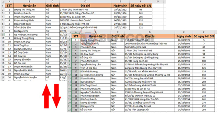
How to reverse data in a column on Excel: Excel is one of the most popular data management tools today. To understand and use Excel effectively, you need to know basic skills such as sorting, filtering, and reversing data. In this article, we will focus on the skill of reversing data in a column on Excel.
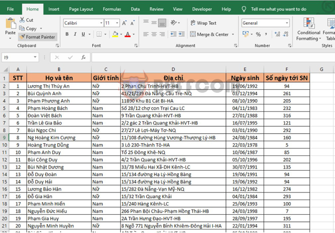
For example, we have a data table as shown below. The requirement is to sort each person’s order by the number of days to their upcoming birthday from smallest to largest. To do this, please follow these steps:
How to reverse data in a column on Excel
Step 1
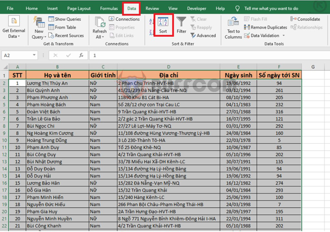
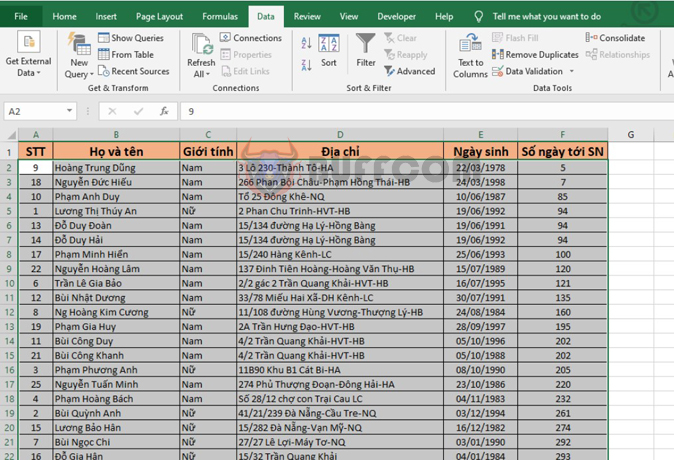
First, you need to select the entire data range, but do not include the header row. Then, select the Data tab on the toolbar, and click the Sort button in the Sort & Filter section.
How to reverse data in a column on Excel
Step 2
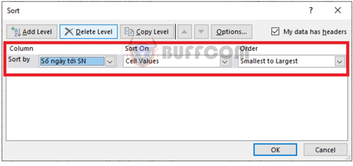
At this point, the Sort window appears. Now, set the options as follows:
- Under the Sort by section, select the Days to BD column, which contains the number of days to the upcoming birthdays that we need to sort.
- Under the Sort On section, select Cell Values, meaning to sort based on the cell values.
- Under the Order section, select Smallest to Largest, meaning to sort from smallest to largest values.
Finally, click OK to complete.
How to reverse data in a column on Excel
That’s it, our data has been sorted by the number of days to the upcoming birthdays from smallest to largest.
How to reverse data in a column on Excel
Step 3
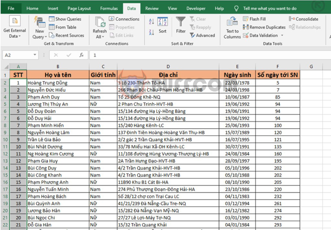
The last step is to enter the order numbers from 1 to the end by entering the first two cells and then dragging the mouse to the end.
How to reverse data in a column on Excel
Those are the basic skills of how to reverse data in a column on Excel that we have shared. However, to use Excel effectively, you need to master many other skills such as calculation, data formatting, report creation, and more. We hope this article helps you work on Excel more easily and efficiently.


