10 ways to use Paste feature in Excel

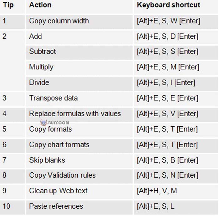
10 ways to use Paste feature in Excel. The Paste Special command appears in most office applications, but perhaps Excel users benefit from it the most. By using this basic feature, as well as other Paste options, users can perform common tasks as well as more complex issues. These tricks are easy to perform and you will definitely use them more once you know about them. In Excel 2007 and 2010, Paste is located in the Clipboard group on the Home tab. In Excel 2003, Paste Special is in the Edit menu. For those who use keyboard shortcuts, we have a table at the end of the article, which includes shortcut keys to perform common actions.
1.Copy column width paste feature
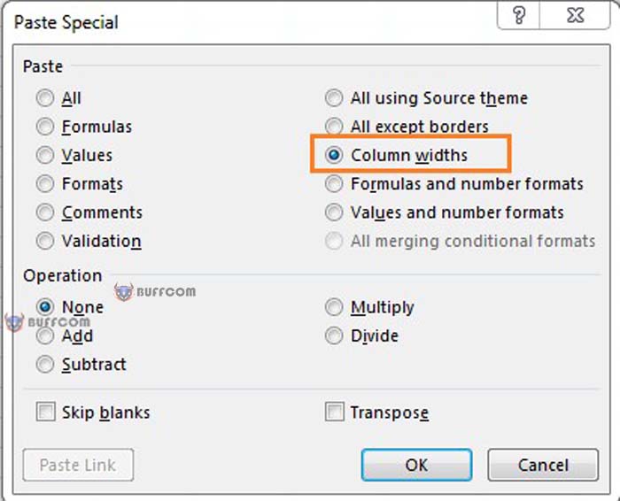
When copying data to a new column, the length of the column will not automatically adjust to fit the new value. With just one more click, you can copy the original width of the column to the target column:
Select the data to be copied and press Ctrl + C to copy the selected value to the Clipboard.
Select a cell in the target column.
On the Home tab, select Paste in the Clipboard group and select Keep Source Column Widths. This option will require one more step when using Excel 2007: Select Paste Special from the drop-down Paste menu. Next, select Column Widths in the Paste section and OK.
Excel will copy the original width of the column to the target cell.
10 ways to use Paste feature in Excel
2.Perform calculations
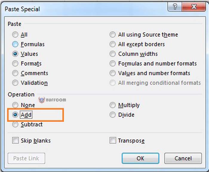
Users can use Paste Special to add, subtract, multiply, and divide. Just enter the number and press Ctrl + C. Then, select the value you want to change with the newly entered number and select Paste Special in the Clipboard group. In the result window, select the appropriate calculation and press OK. Excel will perform the corresponding action using the value you just copied to the Clipboard. Users can also perform calculations with multiple values. Use the same process as above, but copy a range of values instead of just one. Excel will not notice the size if it is not enough, it will only perform the calculations in the order of the values copied.
10 ways to use Paste feature in Excel
3.Swap data
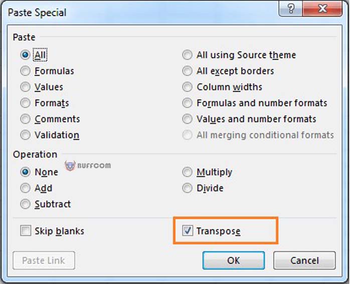
Excel provides users with the swap feature, but sometimes Paste Special is faster to perform this task. Select the source data and perform the following actions:
Press Ctrl + C to copy the data to the Clipboard.
Select the top-left cell of the target row.
Select the Home tab (if necessary) and select Transpose from the drop-down Paste menu.
That’s what users need to do. From now on, you can copy a column of data to a row and vice versa.
10 ways to use Paste feature in Excel
4.Replace the formula with the calculated result
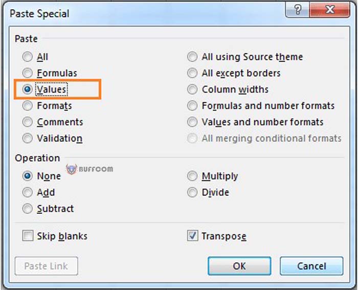
Sometimes, users may want to replace the formula with its actual value. For example, you may want to replace a series of RAND() functions with their values instead of allowing the formula to calculate itself. This is a common task for Paste Special. To copy the formula with its value, follow these steps:
Select a range of formulas and then press Ctrl + C.
In the Clipboard group, select the drop-down Paste menu.
Select Values.
Do this to replace formulas with their actual values. Before using this method, you may want to back up your work as a precaution.
10 ways to use Paste feature in Excel
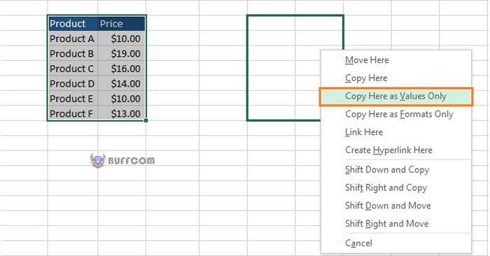
Trick to use the mouse to perform the task:
Select the range.
Right-click on the border and drag the range to the adjacent column (or row).
Drag the selected range back to the source. This will prompt Excel to display the shortcut menu without moving the selected values.
Select Copy Here As Values Only.
5.Copy formatting paste feature.
Most of us use Format Painter to copy formatting from one cell to another or to a row. However, when using Format Painter with an entire column or row, it can be somewhat inconvenient. Here’s how to use Paste Special to replace it:
Select the cell containing the format you want to copy and press Ctrl + C.
Select within the column or row you want to format. (Press Ctrl + Spacebar to select the entire column or Shift + Spacebar to select the entire row).
For the selected column or row, select Formatting from the drop-down Paste menu in the Clipboard group. Excel 2007 requires an additional step: Select Paste Special from the drop-down Paste menu, select Formats in the Paste section, and click OK.
10 ways to use Paste feature in Excel
6.Copy chart formatting paste feature.
Users may have to spend a lot of effort to format the chart to make it look beautiful and then have to do all the same work with a different type of data. In this case, do not reformat the new chart, use Paste Special. This assumption is similar to step 5, but the steps are slightly different:
Select the chart with the format you want to copy and press Ctrl + C.
Select the chart you want to format and then select Paste Special from the drop-down Paste menu. Excel will display the Paste Special dialog box, with three options.
Select Formats and click OK.
Excel reacts differently when copying chart formats, but it can easily complete the task.
7. Skip a range of empty cells
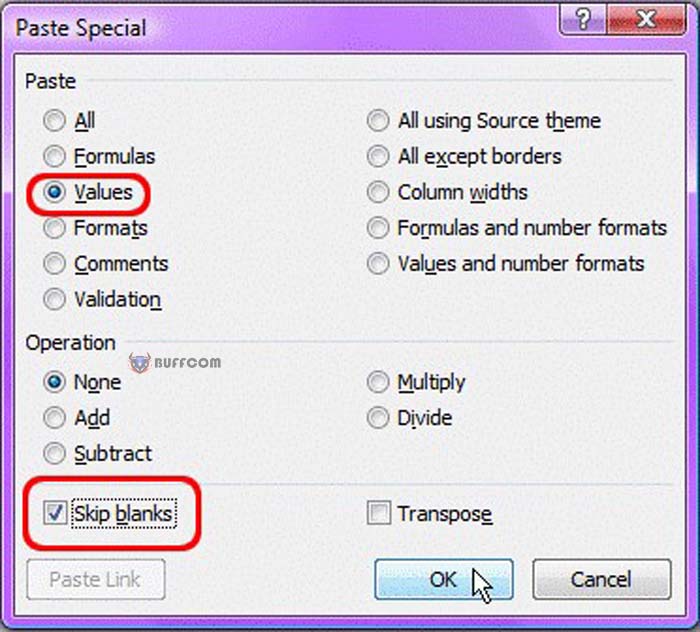
Using the Skip Blanks option, you can replace the current value while still skipping cells that have no value in the original data. In other words, if there is an empty cell in the original data and a value in the corresponding paste range, this option will not replace the current value with an empty cell. You can use it with all other options:
Select the original data range and press Ctrl + C.
Select the top left cell in the destination range.
From the drop-down Paste menu, choose Paste Special.
Select Skip Blanks and click OK.
Excel will not overwrite the current value with an empty cell.
10 ways to use Paste feature in Excel
8.Copy Data Validation Paste feature.
After spending time setting up Data Validation rules or lists to improve data entry, you may want to apply similar rules to other cells or ranges. The good news is that you don’t have to repeat all the steps above. Using Paste Special, you can simply copy and paste:
Select the cell containing the Data Validation rule and press Ctrl + C.
Select the target cell to paste to.
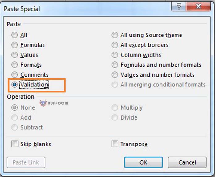
From the drop-down Paste menu, choose Paste Special.
Select Validation and click OK.
Setting up Data Validation can be tedious and time-consuming; Paste Special is much easier!
10 ways to use Paste feature in Excel
9. Removing text formatting on the web
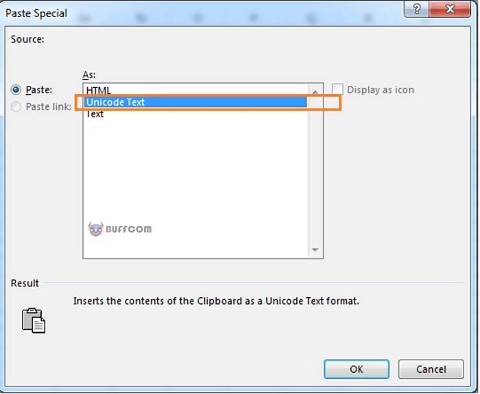
When copying text from the web, you may encounter issues with Excel retaining the original formatting. Generally, this is not what you want. If you have enabled Excel’s Show Paste Options feature (located in the Advanced tab of the Excel Options dialog box), you will see the Clipboard icon immediately after pasting the text into the worksheet. Users can select Match Destination Formatting from the Clipboard drop-down menu to remove unnecessary formatting. If you are using Excel 2013, you will definitely appreciate using this Paste Special solution:
10 ways to use Paste feature in Excel
10.Copy the text from the web.
In Excel, select where you want to insert the text.
Select Paste Special mode from the drop-down menu and choose Unicode Text.
Use this option to copy external data, not just web text, into Excel.
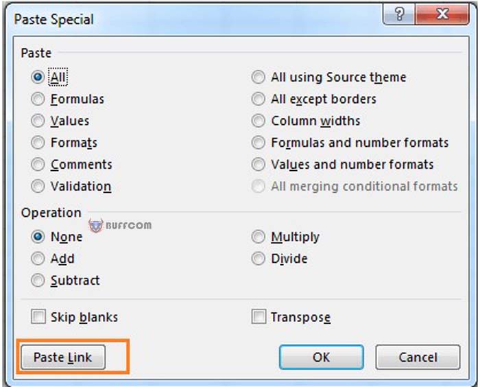
Paste link
Users can reference a cell by referencing the cell address with an equal sign. For example, enter =A1 to return the contents of cell A1. Usually, we use these references in larger expressions and formulas. Occasionally, we still reference a cell with itself. Paste Link can help when referencing multiple cells:
Select the range to reference and press Ctrl + C.
Select the target cell and press Paste Link from the Paste drop-down menu.
10 ways to use Paste feature in Excel
Using Paste Link is faster than manual referencing. Shortcuts for paste actions:
10 ways to use Paste feature in Excel


