Tips to lock the header of a table in Excel
Tips to lock the header of a table in Excel: When working on Excel, sometimes you may encounter a long table with too much data, making it difficult for you to reference cells in the header area. At this point, we need to lock the header area to make it easier to reference. If you don’t know how to lock the header area of a table in Excel, please follow the instructions in this article.
Step 1
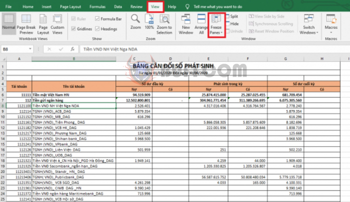
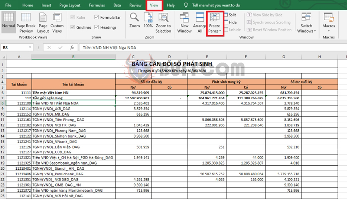
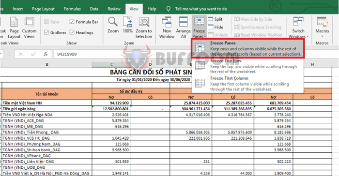
To lock the header of the table, first you need to open the Excel file containing the worksheet that you want to lock the header for. Then select the View tab on the toolbar. Next, click on the Freeze Panes icon in the Window section.
 Step 2
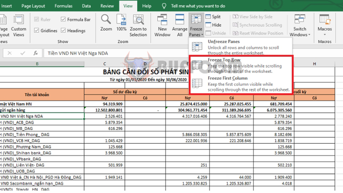
At this point, the scroll bar of the Freeze Panes section will appear. If your header is only the first row or the first column, you can choose one of the following two options to quickly lock the header:
- Freeze Top Row: locks the top row of the workbook
- Freeze First Column: locks the first column of the workbook
 Step 3
If you want to lock more than one row and column, you need to place the mouse pointer on the first cell in the next column of the columns that you want to lock, and on the first cell of the row below the rows that you want to lock. For example, if you want to lock the Debit and Credit rows and the Account Name column in the table above, you need to place the mouse pointer at cell C6. Then select the View tab and click on the Freeze Panes icon. The scroll bar appears and you select Freeze Panes.
 So, this article has guided you on how to lock the header area of a table in Excel. Hopefully, it will be useful to you in your work. Wish you success!


