Efficient Excel Tutorial: Removing Duplicate Rows in Excel

Efficient Excel Tutorial: Removing Duplicate Rows in Excel. When working with an Excel worksheet, it can be challenging to manage duplicate entries, especially if you are not the original creator of the file. To avoid encountering errors, it is advisable to identify and eliminate any duplicates in the worksheet.

This article presents two effective methods to help you remove duplicates from your Excel worksheets.

Removing Duplicates with Conditional Formatting

This method is useful when you need to selectively remove some duplicates while keeping others. Here’s a step-by-step guide:

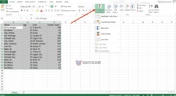
Step 1: Highlight the entire table by pressing CTRL + A. Next, go to the Home tab and select “Conditional Formatting”.

Efficient Excel Tutorial: Removing Duplicate Rows in Excel

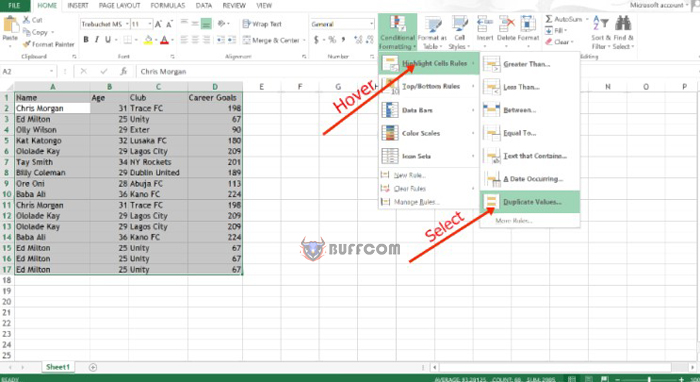
Step 2: Go to the “Highlight Cell Rules” option and choose “Duplicate Values”.

Efficient Excel Tutorial: Removing Duplicate Rows in Excel

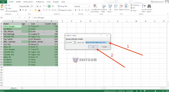
Step 3: Choose how you want the duplicates to be highlighted and click “Ok”.

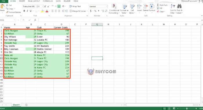
The duplicate cells will now be highlighted, so you can remove any unnecessary ones manually. Note that some duplicates may still be useful.

Removing Duplicates in Excel using the Remove Duplicate Command

Step 1: Go to the “Data” tab and click on “Remove Duplicates”.

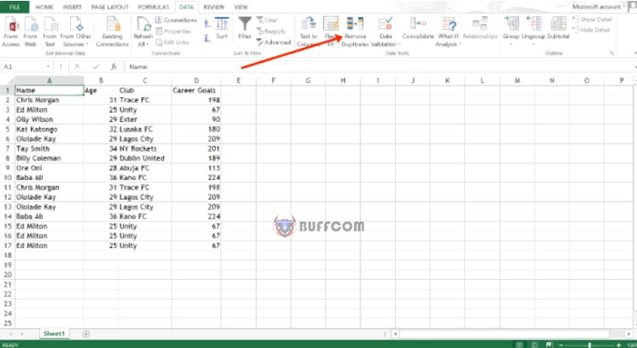
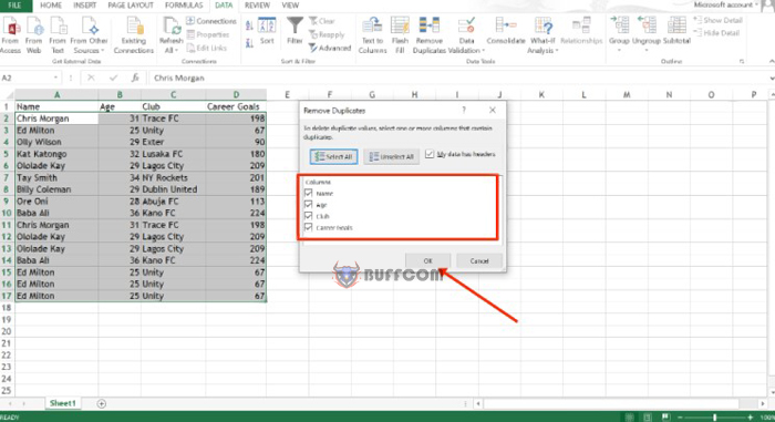
Step 2: Select all the columns in the table and click “Ok”.

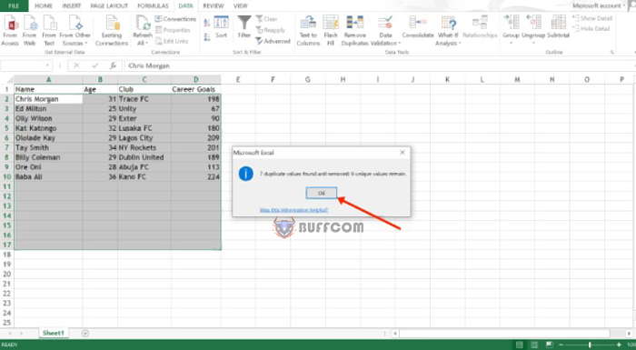
Step 3: A message will appear confirming that duplicates have been removed. Click “Ok” to close it.

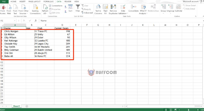By removing duplicates, you can improve your Excel productivity. If you found this article helpful, please share it with others. Thank you for reading!