Calculate the Sum of All Nth Rows In Excel

Calculating the sum of all rows is easy, but what if you need to calculate the sum of all Nth rows in Excel, for example, calculate the sum of the 5th rows in a table? Let Buffcom.net show you how!
3 Steps to Write an Array Formula to Calculate the Sum of All Nth Rows in Excel
To calculate the sum of all Nth rows in Excel, we need to use an array formula. An array formula is a formula that can perform multiple calculations on one or more items in an array. (An array can be a row, a column, or a range that combines multiple rows and columns). An array formula can return multiple results or a single result.
In the example used below, we will calculate the sum of the 2nd rows in the table, i.e., N = 2. Let’s go through each step to write a nested function.
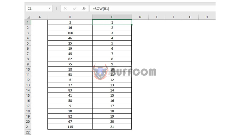
Step 1: Use the ROW Function to Return the Number of Rows in a Cell
The ROW function returns the row number of a cell or range of cells that you enter in the formula. The returned value will be a specific number with the position on the column.
To determine the row of a cell, you enter the formula:
=ROW(reference range)
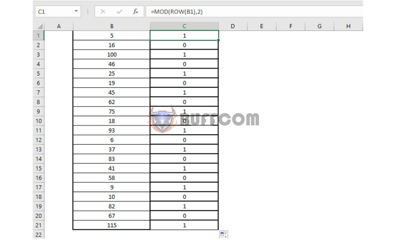
 Step 2: Use the MOD Function to Indicate the Characteristics of N
The MOD function will return the remainder of a division.
In this example, for the second row, MOD(2,2) = 0 because 2 divided by 2 equals 1 with a remainder of 0. As a result, the formula returns 0 for all 2nd rows. So, in the case of calculating the sum of all 2nd rows in Excel (N=2), we need to find the rows that have a remainder of 0 when divided by 2.
The formula now is: =MOD(ROW(reference range),N)
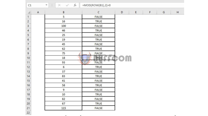
 Change the formula a little to =MOD(ROW(cell reference),N)=0 to replace the remainder with TRUE or FALSE. In this example, any rows with a number that is divisible by 2 will return TRUE, and these are the rows we need to calculate the sum of.
 Step 3: Calculate the Sum of All Nth Rows in Excel Using the SUM Function
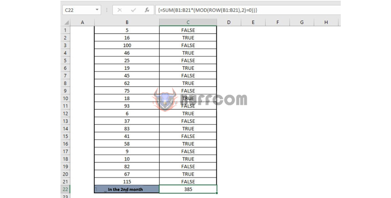
To calculate the product sum of these two ranges (in this case, FALSE = 0, TRUE = 1, depending on the situation and can be changed accordingly), use the SUM function:
=SUM(reference range*(MOD(ROW(reference range),N)=0)
After writing the formula in the sum cell, press the CTRL + SHIFT + ENTER combination to return the result.
 Note: After pressing Ctrl + Shift + Enter, the formula bar will indicate that this is an array formula by automatically placing it in curly braces {}. So, press the combination keys instead of typing these braces manually. They will disappear when you edit the formula.
If you are using Office 365 or Office 2021, you don’t need to press the combination keys, just press Enter, and the formula will not have curly braces.
Explanation
The product of these two ranges (constant array) is stored in Excel memory, not in a range. The constant array in Excel will look like:
{0; 16; 0; 46; 0; 19; 0; 62; 0; 18; 0; 6; 0;83; 0; 58; 0; 10; 0; 67; 0}
This constant array is used as an argument for the SUM function, which returns the result of 385.
Conclusion
Through this article, Buffcom.net has instructed you on how to write an array formula to quickly calculate the sum of the Nth rows in Excel.
3 steps to write a formula to calculate the sum of all Nth rows in Excel:
B1: Use the ROW function to return the row number of the cell.
B2: Use the MOD function to identify the Nth rows.
B3: Calculate the sum of the Nth rows using the SUM function.
In addition, if your job is related to Office computing but the software does not meet your needs. To purchase genuine software, please contact Buffcom.net for support!


