2 methods to display negative numbers in red in Microsoft Excel

2 methods to display negative numbers in red in Microsoft Excel. When entering a negative value into a Microsoft Excel spreadsheet, you can precede the value with a hyphen character (-) to indicate the “negative sign”. However, in many cases, you may not want to display this character. Instead, you might prefer Excel to automatically display negative values in red or with parentheses. There are two ways to achieve this: using a format and using conditional formatting.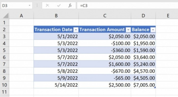

The first method is simple and quick, as Excel provides built-in formats specifically designed for displaying negative values. The second method is useful when you are already using a format that doesn’t handle negative values correctly. Although this may not be a common issue, it’s good to know that there is an alternative method available if needed.

2 methods to display negative numbers in red in Microsoft Excel.

Using a format:

One traditional and easy way to display negative values in red is by applying a format in Excel. Fortunately, Excel offers a built-in format that automatically displays negative numbers in red. Here’s how you can use it:

1. Select the range of currency values in your Excel sheet.
2. On the Home tab, click on the dialog launcher in the Number group. In Excel for the web, choose “More Number Formats” from the Number dropdown.
3. In the resulting window, select the “Currency” category from the list. If you have already assigned a Currency format, Excel will select it for you. There are four formats available for negative numbers.
4. Choose the last format, which displays the number in red and wrapped in parentheses.

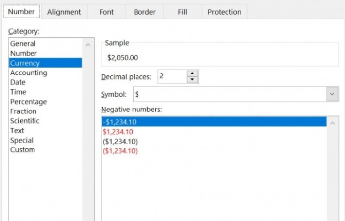
By applying this format, negative values (such as debits) will be displayed in red and wrapped in parentheses. Users can still enter negative values by preceding them with a hyphen character, but the format will not display the hyphen. This format can be applied to the desired range of cells.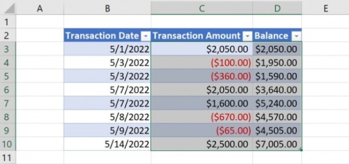

Using conditional formatting:

In cases where a simple format is not sufficient or you have already applied a different format, you can use conditional formatting to display negative values in red. Here’s how:

1. Select the range of cells that you want to apply the conditional format to.
2. On the Home tab, click on “Conditional Formatting” in the Styles group.
3. Choose “New Rule” from the dropdown menu.
4. In the resulting window, select the option “Use a Formula to Determine Which Cells to Format”.
5. Enter the formula “=C3<0” in the lower pane. Adjust the cell reference according to your selection.
6. Click on “Format”.
7. In the Format window, go to the “Font” tab and choose the color red from the dropdown.
8. Click “OK” to apply the format.

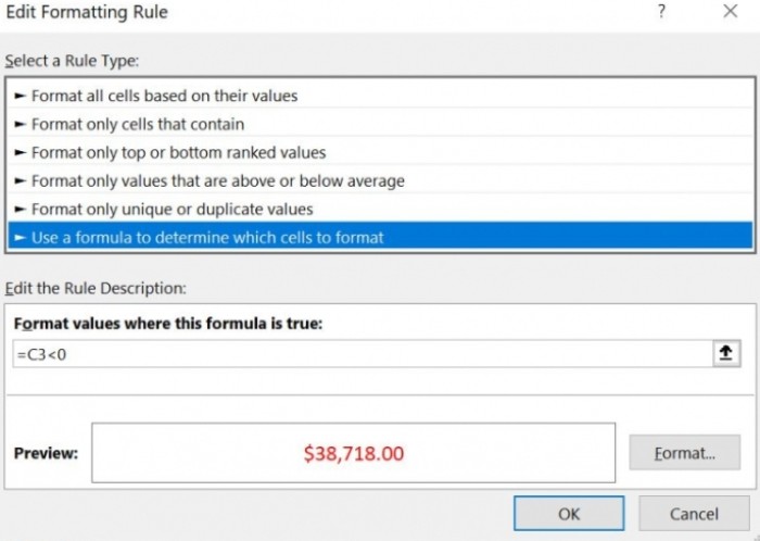
With this conditional format, any values in the selected range that are less than 0 (indicating negative numbers) will be displayed in red. However, unlike the format method, the values will not be wrapped in parentheses.

While the built-in format method is usually the preferred choice, the conditional formatting method can be used when necessary. It’s always helpful to have alternatives available.

Continuing from the previous response:

It’s worth noting that both methods mentioned above are applicable in Microsoft Excel and provide different options for displaying negative numbers in red. The format method is suitable when you want a consistent display across a range of cells with a predefined format, while conditional formatting allows for more flexibility and customization based on specific conditions.

Using these methods, you can enhance the visual representation of negative numbers in your Excel spreadsheets, making it easier to distinguish them from positive values. This can be particularly useful when working with financial data, budgets, or any other scenarios where negative numbers play a significant role.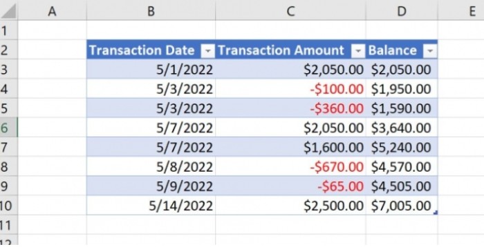

Remember to choose the method that best suits your needs and aligns with the formatting requirements of your Excel sheet. By utilizing these techniques, you can effectively manage and present negative numbers in a visually appealing and intuitive manner within your Excel workbooks.