How to Find the Cell with the Maximum Value in a Column in Microsoft Excel

How to Find the Cell with the Maximum Value in a Column in Microsoft Excel. In this article, we will explore how to find the maximum value in a column that meets multiple conditions in Microsoft Excel.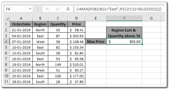

Scenario: When working with large data ranges, it is often necessary to find the maximum value within a range where multiple conditions are met. In other words, we want to find the maximum value using the Excel IF function. The IF function returns True or False, and the MAX function looks for the maximum value from the corresponding array.

How to Find the Cell with the Maximum Value in a Column in Microsoft Excel

Syntax to find the maximum value with multiple criteria: {=MAX(IF(Criteria1=Match1), IF(Criteria2=Match2, Range_Max))}

Note: When working with arrays or ranges in Excel, use Ctrl + Shift + Enter. This will automatically generate curly braces around the formula. Do not manually insert these curly braces.

Example: To better understand the concept, let’s test this formula using the example provided below. We will apply the formula to values with specific criteria.

Use the formula: {=MAX(IF(B2:B11=”East”, IF(C2:C11 > 50, D2:D11)))}

Criteria 1: Price must be from the region “East.” Criteria 2: Price where quantity is greater than 50.

Explanation: The expression IF(C2:C11 > 50, D2:D11) returns an array of FALSE values and price values where the quantity is greater than 50: {FALSE; 303.63; 108.46; 153.34; FALSE; 95.58; 520.01; 90.27; 177; FALSE}

The expression IF(B2:B11=”East”, IF(C2:C11 > 50, D2:D11)) returns an array of price values where the region is East and the quantity is greater than 50.

The MAX function finds the maximum value from the returned array, which is the required price value.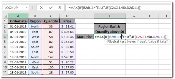

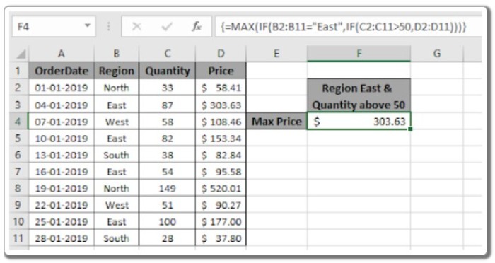
By matching the range (B2:B11) with the value “East” and the quantity range (C2:C11) with values greater than 50, we obtain the maximum value from the price range (D2:D11). Press Enter to get the maximum value from the range.

As you can see, we have obtained the maximum value if the criteria match within the range of values.

Alternative function for Excel 365 and 2019 versions: The Excel MAXIFS function is a new function introduced in Excel 365 and 2019. This function returns the maximum value from a given range based on specified criteria.

Syntax of the MAXIFS function: =MAXIFS(max_range, criteria_range1, criteria1, …)

Max_range: The numeric range that contains the maximum value. Criteria_range1: The range that you want to filter before obtaining the maximum value. Criteria1: The criteria or filter to be applied to criteria_range before obtaining the maximum value. You can have multiple pairs of criteria_range and criteria.

Let’s understand the MAXIFS function with an example:

How to Find the Cell with the Maximum Value in a Column in Microsoft Excel

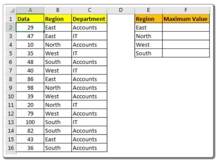
Example: Here, we have a table of data. The first column contains numeric values, the second column contains regions, and the third column contains departments. Our task is to find the maximum value from the first range for each region.

The formula to obtain the maximum value from the “East” region will be: =MAXIFS(A2:A16, B2:B16, “East”)

This formula will return 82.

In this example, we used a hardcoded criteria, but we can also use a reference for the criteria to make it dynamic. =MAXIFS($A$2:$A$16, $B$2:$B$16, E2)

Here, absolute ranges are used to lock the maximum range and criteria range

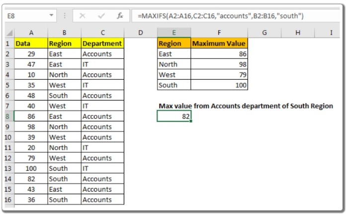
You can add multiple criteria in the MAXIFS function. For instance, if you want to find the maximum value from the IT department in the South region, the formula would be:

=MAXIFS(A2:A16, C2:C16, “IT”, B2:B16, “SOUTH”)

How to Find the Cell with the Maximum Value in a Column in Microsoft Excel

This formula will return 100 based on the provided data. If you replace “IT” with “Accounts,” the MAXIFS function will return 82.

So, this article discussed how to use the MAXIFS function in Excel 365 and 2019. I hope you found it helpful. If you have any doubts or questions about this article or any other Excel topic, feel free to ask in the comments section below.