The Double Negatives (–) in Excel

The Double Negatives (–) in Excel. In advanced Excel formulas, you may have come across the use of double negative signs (–) in some situations. These double minus signs serve a specific purpose in Excel formulas, especially when working with boolean values.
The primary function of double negatives is to convert boolean values into binary values. Specifically, they are used to transform TRUE and FALSE values into 1s and 0s, respectively. This is particularly useful when working with array functions and complex formulas in Excel. Let’s look at an example to understand this better.
The Double Negatives (–) in Excel
Example:
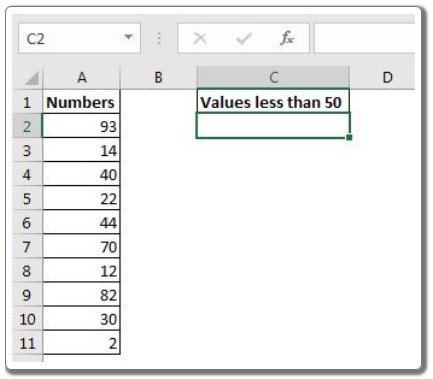
Suppose we have a list of numbers, and we want to count how many of them are less than 50. While the COUNTIF function can easily achieve this, let’s use the SUMPRODUCT function to learn about the double minus symbol in Excel formulas.
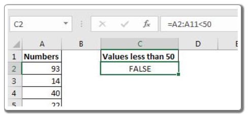
- Write the following formula in cell C2: =A2:A11<50

When you hit enter, it will display “FALSE.” However, the formula is actually returning an array of TRUE and FALSE values, which you can verify by selecting the formula in edit mode and pressing the F9 key. The array will look like this: {FALSE;TRUE;TRUE;TRUE;TRUE;FALSE;TRUE;FALSE;TRUE;TRUE}, where TRUE represents values less than 50 in the range A2:A11.
- To convert these boolean values into 1s and 0s, add the — sign before the statement: =–(A2:A11<50)
Now, when you hit enter, it will show “0” because the first value in the array is not less than 50. But if you use the debugging key F9, you will see an array of 1s and 0s: {0;1;1;1;1;0;1;0;1;1}, where each TRUE value is represented by 1.
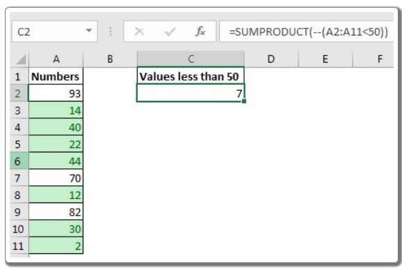
- To count the number of values that are less than 50, wrap the formula inside the SUMPRODUCT function: =SUMPRODUCT(–(A2:A11<50))
The formula will sum up the array returned by the internal statement, and in this case, the result will be 7.
If you were to remove the double negatives (–), and make the formula =SUMPRODUCT((A2:A11<50)), it would return 0. This is because the array returned by A2:A11<50 contains boolean values, and the SUMPRODUCT function cannot directly sum boolean values.
Alternative ways to achieve the same result of converting boolean values into binary values include adding 0 to boolean values, multiplying them by 1, or using the N function:
=SUMPRODUCT((A2:A11<50)+0) =SUMPRODUCT((A2:A11<50)*1) =SUMPRODUCT(N(A2:A11<50))
All of the above formulas will accomplish the task. While the double minus sign (–) is one way to perform this conversion, there are other valid alternatives as well. The use of double negatives was illustrated in this simple scenario, but in more complex situations, you may encounter situations where you need to convert boolean values into binary values, and these techniques can be helpful.


