VLOOKUP for Automatic Discount in Data Validation
How to Use VLOOKUP Function in Data Validation for Automatic Discount Calculation
VLOOKUP for Automatic Discount in Data Validation
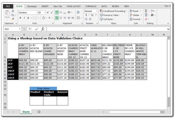
How to Use VLOOKUP Function in Data Validation for Automatic Discount Calculation. I’m currently working on a spreadsheet that displays various discounts for products based on the quantity purchased. To achieve this, I’ve set up a data validation dropdown list that lists the required quantities (e.g., 1 case, 2 cases, etc.), and I have another sheet containing all the relevant data. In this sheet, column A represents the case quantity, column B has the product name in cell B1, and subsequent cells in column B contain discounts corresponding to the case quantities in column A. My goal is to have the discount amount on Sheet 2 automatically populate based on the selections made in Sheet 1.
Here’s how to accomplish this:
Step 1: Create the dropdown list for the product and product code:
Select cell C15.
Navigate to the Data tab, click on Data Validation, and then select Settings.
In the Allow dropdown, choose List.
In the Source field, input the range containing your product names (e.g., B4:L4).
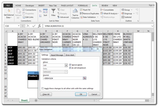
VLOOKUP for Automatic Discount in Data Validation
Step 2: Create the dropdown list for the quantity:
Select cell D15.
Again, go to the Data tab, click on Data Validation, and choose Settings.
Set Allow to List.
In the Source field, input the range containing your quantity options (e.g., A5:A10).
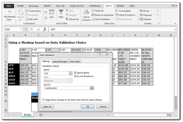
VLOOKUP for Automatic Discount in Data Validation
Step 3: Enter the formula in cell E15 to automatically calculate the discount amount:
In cell E15, input the following formula:
=INDEX($A$4:$L$10, MATCH(D$15, $A$4:$A$10, 0), MATCH(C15, $A$4:$L$4))
After entering the formula, press Enter.
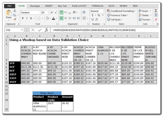
VLOOKUP for Automatic Discount in Data Validation
Now, whenever you change the product or quantity from the dropdown lists, the discount amount in cell E15 will update automatically based on the information in your data.

