Exploring Advanced Techniques for Conditional Formatting in Excel

Exploring Advanced Techniques for Conditional Formatting in Excel
Introduction:
Exploring Advanced Techniques for Conditional Formatting in Excel
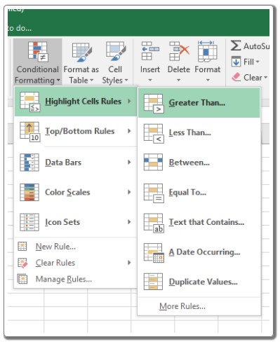
Exploring Advanced Techniques for Conditional Formatting in Excel. In this article, we will delve into advanced methods of utilizing Conditional Formatting in Microsoft Excel. Despite Excel’s remarkable capabilities, some functionalities may not be immediately apparent. One such feature is Conditional Formatting, a tool used to format cells or ranges based on specific conditions. This tool can be applied to cell values or formulas. For instance, you can utilize Conditional Formatting to highlight cell values based on criteria defined by formulas or specific values within a range.
Exploring Advanced Techniques for Conditional Formatting in Excel
Conditional Formatting Possibilities:
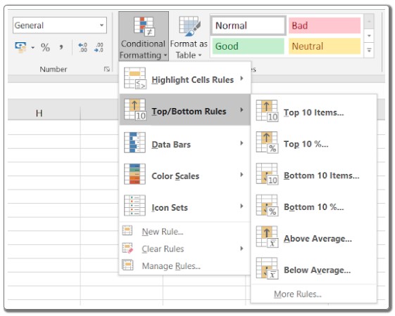
Conditional Formatting offers a wide array of possibilities for enhancing data presentation. These include highlighting numbers in ascending or descending order, targeting specific values or dates, and employing various formatting techniques such as cell background colors, font colors, data bars, color scales, and icon sets.
Exploring Further Conditional Formatting in Excel:
Let’s delve into some scenarios that demonstrate how to leverage Conditional Formatting in Excel for day-to-day data management tasks:
Highlighting a Cell Based on Another Cell:
Conditional Formatting can be employed to format cells based on conditions in other cells. For instance, you might want to format certain cells based on whether another cell meets a specific condition. To achieve this, follow these steps:
Exploring Advanced Techniques for Conditional Formatting in Excel
Select the column containing the IDs you wish to format.
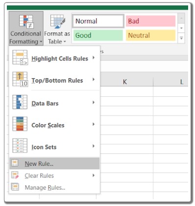
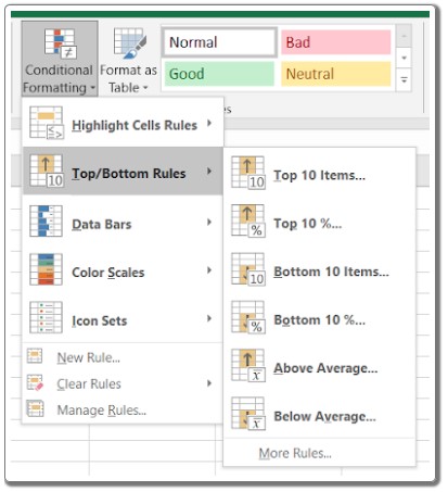
Navigate to the “Conditional Formatting” menu and choose “New Rule.”
In the rule creation dialog, select “Use a formula to determine which cells to format.”
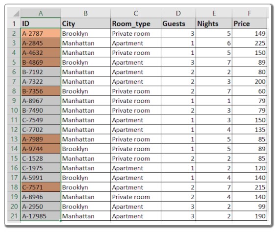
Enter the formula: =E2>=5
Exploring Advanced Techniques for Conditional Formatting in Excel
Customize the formatting style as needed (e.g., changing background color to orange).
Confirm your settings in the preview and click “OK.”
Conditional Formatting Based on Dates:
Exploring Advanced Techniques for Conditional Formatting in Excel
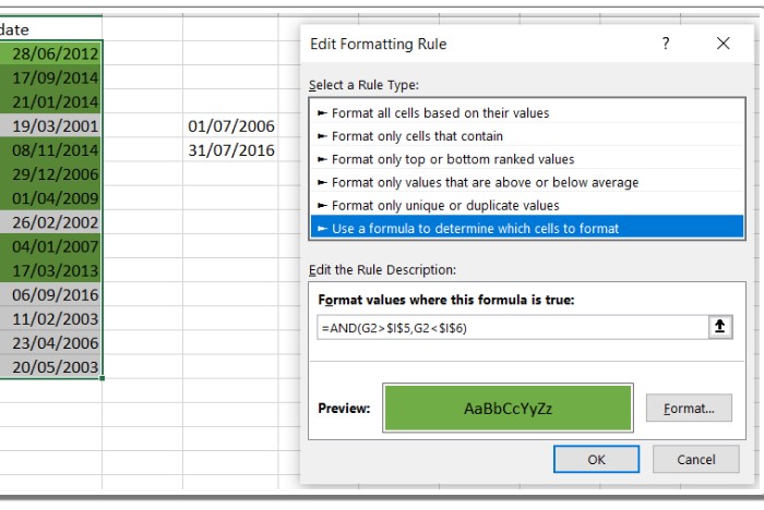
Treating dates as numerical values, Conditional Formatting can be used to format cells between specific date ranges. To do this:
Choose the cells containing the dates.
Access the “Conditional Formatting” menu and select “New Rule.”
Opt for “Use a formula to determine which cells to format.”
Input the formula: =AND(G2>$I$5, G2<$I$6)
This formula checks if a date falls between two given dates.
Adjust formatting options to match your requirements.
Concealing Zeros Using Conditional Formatting:
Exploring Advanced Techniques for Conditional Formatting in Excel
You can use Conditional Formatting to hide zero values in a table by making them blend into the background color. Here’s how:
Highlight the data range.
Go to “Conditional Formatting,” then “Highlight Cells Rules,” and choose “Equal To.”
Set the value to 0 and modify the font color or background color to match the cell color.
These are just a few examples of the advanced techniques you can apply using Conditional Formatting in Excel. By understanding how to create, edit, and delete conditional formatting rules, you can efficiently manipulate the appearance of your data based on specific conditions. Remember, formulas used in Conditional Formatting should be tested beforehand in cells to avoid potential errors.
Conclusion:
In summary, Conditional Formatting is a potent tool within Excel that allows for dynamic and visually appealing data representation. By mastering these advanced techniques, you can enhance your data management skills and efficiently highlight, format, and manipulate data based on various conditions.

