• Microsoft Office
  • Microsoft Windows
  • Other Software
  • Anti Virus
  • Blog
    • Word
    • Excel
    • Powerpoint
    • Software tricks/tips
  • POLICIES
    • PAYMENT GUIDE
    • SHIPPING POLICY
    • REFUND POLICY
    • TERMS & CONDITIONS
    • Contact Us

No products in the cart.

  • Microsoft Office
  • Microsoft Windows
  • Other Software
  • Anti Virus
  • Blog
    • Word
    • Excel
    • Powerpoint
    • Software tricks/tips
  • POLICIES
    • PAYMENT GUIDE
    • SHIPPING POLICY
    • REFUND POLICY
    • TERMS & CONDITIONS
    • Contact Us

No products in the cart.

  • Microsoft Office
  • Microsoft Windows
  • Other Software
  • Anti Virus
  • Blog
    • Word
    • Excel
    • Powerpoint
    • Software tricks/tips
  • POLICIES
    • PAYMENT GUIDE
    • SHIPPING POLICY
    • REFUND POLICY
    • TERMS & CONDITIONS
    • Contact Us

No products in the cart.

  • Microsoft Office
  • Microsoft Windows
  • Other Software
  • Anti Virus
  • Blog
    • Word
    • Excel
    • Powerpoint
    • Software tricks/tips
  • POLICIES
    • PAYMENT GUIDE
    • SHIPPING POLICY
    • REFUND POLICY
    • TERMS & CONDITIONS
    • Contact Us
Excel

How to Create a Horizontal Filter in Excel

0 Comments

To apply a horizontal filter in Excel, you can use the FILTER function, which allows you to filter a table based on specified criteria. By specifying the table range and criteria, you can filter data horizontally.

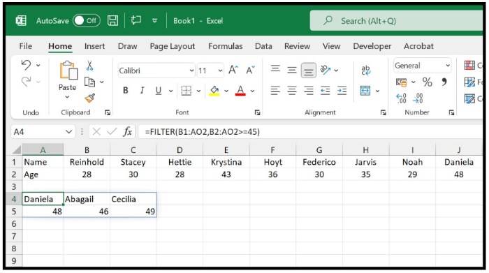
Let’s consider an example where we have a small dataset with names and ages arranged horizontally (headings in rows). Our goal is to filter in Excel the data based on ages above 45.Filter in Excel 1
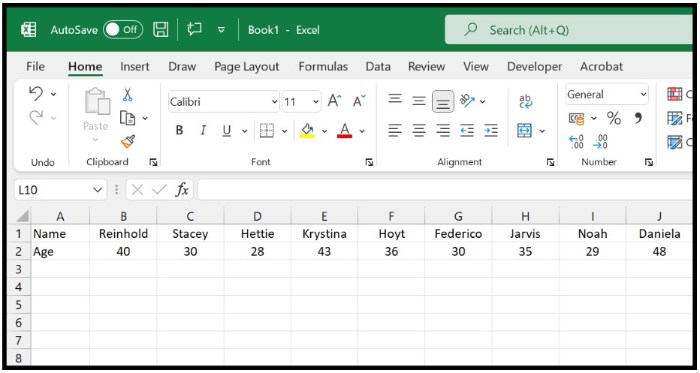
Here’s how you can apply a horizontal filter in Excel:

  1. Start in cell D2 and enter the FILTER function.
  2. In the first argument, refer to the range B2:AO2 where the actual data to be filtered is located.
  3. In the second argument, specify the range where the age values are located.
  4. Add the greater than or equal to (>=) operator after the age range.
  5. Enter the criteria value of 45.
  6. Optionally, in the third argument, specify a value to use for cells where there is no value.
  7. Close the parentheses and press Enter to obtain the filtered data.Filter in Excel 2

The formula to apply the horizontal filter would be:

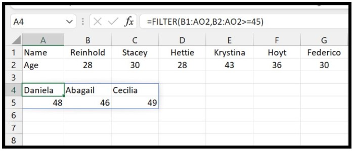
=FILTER(B1:AO2, B2:AO2>=45)

How Does this Formula Work?

The FILTER function is dynamic and enables working with multiple values in a single formula, returning values in multiple cells.

Let’s break down the formula into two parts:Filter in Excel 3
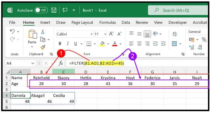
  1. The first part refers to the entire range where names and ages are located (B1:AO2). This tells Excel to consider two separate arrays since we have rows A and B.
  2. The second part only refers to the age column and specifies a condition to test (>=45).

The magic happens in this second part. By specifying the condition, the function tests each value in the age column. In our example, it identifies three values that are greater than or equal to 45, indicating the need to filter those values.Filter in Excel 4
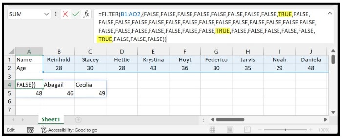
As a dynamic function, selecting any of the filtered cells highlights the entire filtered data. Filter in Excel 5Additionally, you can further manipulate the data by transposing it from horizontal to vertical using the TRANSPOSE function. Simply wrap the FILTER function with the TRANSPOSE function to achieve this.Filter in Excel 6
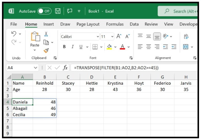
I hope this helps you understand how to create a horizontal filter in Excel.

6
49 Views
How to Concatenate with a Line Break in ExcelPrevHow to Concatenate with a Line Break in ExcelMay 22, 2023
How To Enter Safe Mode In Windows 10May 22, 2023How To Enter Safe Mode In Windows 10Next

Leave a Reply Cancel reply

Your email address will not be published. Required fields are marked *

Recent Posts
  • Retrieve Data Based on Data Validation
    September 7, 2023
    Excel
  • How to Convert Multiple Rows to Columns and Rows in Excel?
    September 6, 2023
    Excel
  • VLOOKUP for Automatic Discount in Data Validation
    September 6, 2023
    Excel
  • How to Convert Text Dates to Dates in Excel?
    September 5, 2023
    Excel
Categories
  • Blog 80
  • Excel 754
  • Powerpoint 36
  • Software tricks/tips 128
  • Uncategorized 8
  • Word 109
Tags
the ISERROR
Top rated products
  • Kaspersky Internet Security 2021 1 year 5 devices key Global Kaspersky Internet Security 2021 1 year 5 devices key Global
    Rated 5.00 out of 5
    $45.00
  • Windows Server 2022 Datacenter Key Global
    Rated 5.00 out of 5
    $15.00
  • Kaspersky Small Office Security 10 PCs + 10 Mobiles + 1 Server 1 Year Kaspersky Small Office Security 10 PCs + 10 Mobiles + 1 Server 1 Year
    Rated 5.00 out of 5
    $164.50
  • Avast Ultimate Suite 2021 1 Year 10 Devices Global
    Rated 5.00 out of 5
    $54.00
  • Windows 11 Pro Key Global
    Rated 5.00 out of 5
    $11.00
Products
  • Buy Office 2021 Professional Plus Key Global For 5 PC
    Rated 5.00 out of 5
    $45.00
  • Buy Office 2021 Professional Plus Key Global Bind To Your Microsoft Account
    Rated 4.83 out of 5
    $49.00
  • Windows Server 2022 Datacenter Key Global
    Rated 5.00 out of 5
    $15.00
  • Windows Server 2022 Standard Key Global
    Rated 4.47 out of 5
    $15.00
  • Windows Server 2022 Remote Desktop Services Device Connections (50) Cal Key Global
    Rated 5.00 out of 5
    $45.00

Buffcom.net always brings the best digital products and services to you. Specializing in Office Software and online marketing services

BIG SALE 50% IN MAY

Microsoft Office
Microsoft Windows
Anti-Virus
Contact Us

Visit Us:

125 Division St, New York, NY 10002, USA

Mail Us:

buffcom.net@gmail.com

TERMS & CONDITIONS | PAYMENT GUIDE  | SHIPPING POLICY  | REFUND POLICY

Copyright © 2019 buffcom.net  All Rights Reserved.