How to Hide and Lock Formulas in Excel
How to Hide and Lock Formulas in Excel. This guide explains how to hide formulas in Excel so that they do not appear in the formula bar. Additionally, you will learn how to quickly lock a selected formula or all formulas on a worksheet to protect them from being deleted or overwritten by other users.
But what if you don’t want your formulas to be displayed in the formula bar or anywhere else on the worksheet, for reasons of confidentiality, security, or other reasons? Furthermore, you may want to protect your Excel formulas to prevent other users from deleting or overwriting them. For example, when sending some reports outside your organization, you may want the recipients to see the final values but not know how to calculate them, without making any changes to your formula.
Fortunately, Microsoft Excel makes it quite simple to hide and lock all or selected formulas on a worksheet, and in this guide, I will provide detailed steps.
How to Hide and Lock Formulas in Excel
You’ve put in a lot of effort in creating a great worksheet that you need to share with others, and you certainly don’t want anyone to mess up any of the formulas that you’ve painstakingly researched! The most common way is to protect the worksheet. However, this not only locks the formulas but also locks all the cells on the worksheet and prevents users from editing any existing cells and entering any new data.
The following steps illustrate how you can only lock selected formulas or all formula-containing cells on a specific worksheet and leave other cells unlocked.
1. Unlock all cells on the worksheet.
How to Hide and Lock Formulas in Excel
To start, unlock all cells on your worksheet. I understand that it may seem confusing because you haven’t locked any cells yet. However, by default, the Locked option is turned on for all cells on any Excel worksheet, whether existing or new. This doesn’t mean that you can’t edit those cells, as locking cells has no effect until you protect the worksheet.
So if you only want to lock cells with formulas, make sure to perform this step and unlock all cells on the worksheet first.
If you want to lock all cells on the worksheet (whether they contain formulas, values, or are blank), then skip the first three steps and go straight to Step 4.
Select the entire worksheet by pressing Ctrl + A or by clicking on the Select All button (gray triangle icon at the top left corner of the worksheet).
Open the Format cells dialog box by pressing Ctrl + 1 or by right-clicking and selecting Format Cells from the context menu.
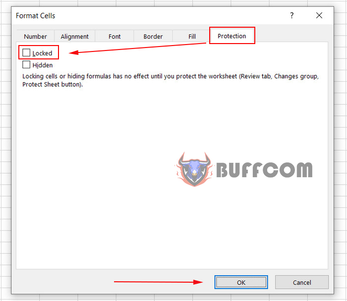
In the Format Cells dialog box, click on the Protection tab.
Uncheck the Locked option and click OK to close the dialog box. This unlocks all cells on the worksheet.
Select the cells containing the formulas that you want to lock. You can do this by dragging the mouse over the cells or by holding down the Ctrl key and clicking on each cell.
Right-click on one of the selected cells and choose Format Cells from the context menu.
In the Format Cells dialog box, click on the Protection tab.
Check the Locked option and click OK to close the dialog box. This locks the selected cells containing formulas. You can verify this by looking at the formula bar, which should display the value of the formula instead of the formula itself.
You can now protect the worksheet to prevent users from editing any cells, including the locked cells containing formulas.
2. Choose the formula you want to lock.
Select the cells containing the formula you want to lock.
To select non-contiguous cells or cell ranges, select the first cell/range, hold down Ctrl, and select the other cells/ranges.
To select all cells containing formulas in the worksheet, do the following:
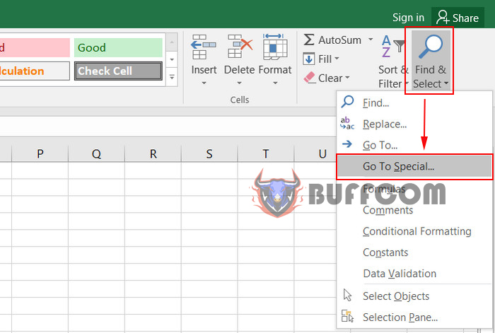
Go to the Home tab > Look in the top right corner > click Find & Select, and select Go To Special.
How to Hide and Lock Formulas in Excel
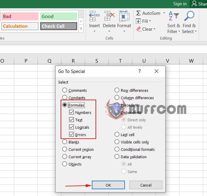
In the Go To Special dialog box, select the Formulas button (this will select all cells containing any type of formula) and click OK.
How to Hide and Lock Formulas in Excel
3. Lock cells using formulas.
How to Hide and Lock Formulas in Excel
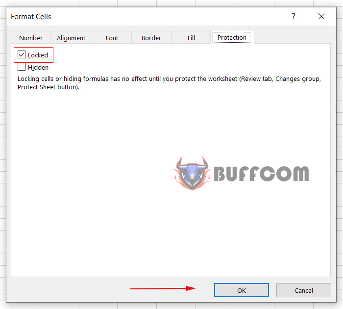
Now, lock the selected cells using a formula. To do this, press Ctrl + 1 to open the Format Cells dialog box, switch to the Protection tab, and select the Locked checkbox.
The lock options prevent users from overriding, deleting, or changing the contents of the cells.
4. Protect the worksheet.

How to Hide and Lock Formulas in Excel
How to Hide and Lock Formulas in Excel
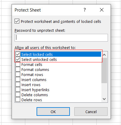
To lock formulas in Excel, selecting the Locked option is not enough because the Locked attribute has no effect unless the worksheet is protected. To protect the worksheet, do the following:
Go to the Review tab > click Protect Sheet.
When the Protect Sheet window appears, enter the password in the corresponding field.
This password is required to remove worksheet protection. No one, including yourself, will be able to edit the worksheet without entering the password, so remember to keep it safe!
Additionally, you need to select the actions that are allowed in your worksheet. As you can see in the screenshot above, two checkboxes are selected by default: Select locked cells and Select unlocked cells. If you click the OK button to only select these two options, users, including yourself, will only be able to select cells (both locked and unlocked) in your worksheet.
If you want to allow other actions, such as sorting, auto-filtering, cell formatting, deleting or inserting rows and columns, check the corresponding options in the list.
Once you have selected any additional actions you want to allow, if any, click the OK button.
The Confirm Password dialog box will appear and ask you to re-enter the password, to prevent an inadvertent typo from locking your Excel worksheet forever. Re-enter the password and click OK.
Done! Your Excel formulas are now locked and protected, even though they are still displayed in the formula bar. If you also want to hide and lock formulas in your Excel worksheet, please read the following section.
Note: If you occasionally need to edit or update your formulas and don’t want to waste time protecting/unprotecting your worksheet, you can move your formulas to a separate worksheet (or even a workbook), hide and lock that worksheet, and then, in your main worksheet, simply refer to the appropriate cells with formulas on that hidden sheet.
How to Hide Formulas in Excel
How to Hide and Lock Formulas in Excel
How to Hide and Lock Formulas in Excel
Hiding formulas in Excel means preventing the formula from being displayed in the formula bar when you click on a cell containing the formula’s result. To hide and lock in Excel, follow these steps:
1. Select a cell or range of cells containing the formulas you want to hide and lock.
You can select non-adjacent cells or ranges by holding down Ctrl or the entire worksheet by pressing Ctrl+A.
2. Open the Format Cells dialog box by performing any of the following actions:
Press Ctrl + 1.
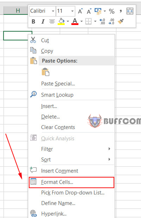
Or Right-click on the selected cell(s) and choose Format Cells from the dropdown menu.
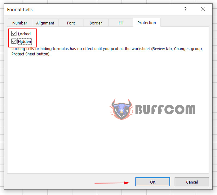
3. In the Format Cells dialog box, switch to the Protection tab and select the Hidden checkbox. This option prevents an Excel formula from being displayed in the formula bar.
The Locked attribute, which prevents the contents of cells from being edited, is selected by default, and in most cases, you want to leave it that way.
4. Click OK.
5. Protect your Excel worksheet by following these steps.
Note: Remember that locking cells and hiding formulas have no effect until you protect the worksheet (a short message right below the Locked and Hidden options in the Format Cells dialog box indicates the next steps). To ensure this, select any cell with a formula and look at the formula bar; the formula should still be there. To truly hide formulas in Excel, make sure to protect the worksheet.
How to Unprotect and Unhide Formulas in Excel
To display formulas that were previously hidden in the formula bar, perform one of the following actions:
Press Ctrl + 1 or right-click on the selected cell(s) and choose Format Cells. Select the Protection tab and uncheck the Hidden checkbox. Then, enter the password you used to protect the worksheet and click OK.
Or Go to the Review tab > click Unprotect Sheet.

How to Hide and Lock Formulas in Excel
Note: If you have hidden formulas before protecting your worksheet, you may want to deselect the Hidden checkbox after removing worksheet protection. This will not have any immediate effect as the formulas will start displaying in the formula bar immediately after you remove worksheet protection. However, if you want to protect the same worksheet in the future but allow users to view the formulas, make sure the Hidden attribute is not selected for those cells (select the cell
This is how you can hide and lock formulas in Excel. In the next tutorial, we will discuss different ways to copy formulas and you will learn how to apply formulas to all cells in a specific column with just one click.

