Instructions for inserting Sparklines in Excel
Instructions for inserting Sparklines in Excel. One of the new features of Excel from version 2010 onwards is the addition of Sparklines. These are small charts that quickly display a selected group of data. Sparklines make it easy to quickly identify unusual data in a flash. This article will guide you through how to insert Sparklines in Excel.
WHAT IS A SPARKLINE IN EXCEL?
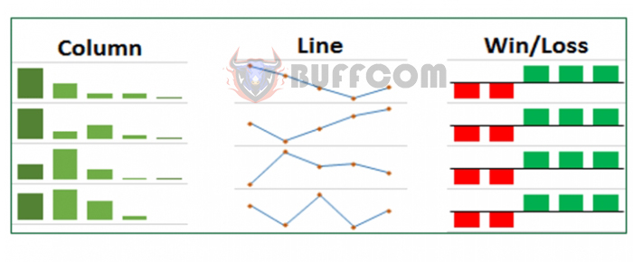
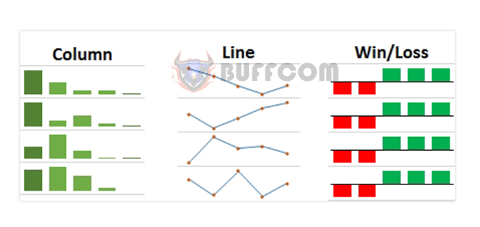
An Excel sparkline is a small chart placed in a single cell. It provides a visual representation of the selected data set. Sparklines allow you to quickly view and analyze relationships, trends for multiple data series at once. There are three types of sparklines: Line, Column, and Win/Loss.
The Line type is a simple line chart in a cell. The Column type is a simple bar chart that reflects the relative size of the value. Win/Loss shows a positive or negative representation of the data set.
Instructions for inserting Sparklines in Excel
WHY SHOULD YOU USE SPARKLINES?
Compared to traditional charts, sparklines provide a different way to display data. They are small and do not take up much space. Sparklines are ideal when you need a clear overview of data without the features of a chart. They are also easy to view and analyze trends on an individual basis. And Sparklines can really help you manage your data.
HOW TO INSERT SPARKLINES IN EXCEL 2010 – 2016
Excel’s sparklines are usually inserted into cells next to the data source. The steps are the same for all types of sparklines.
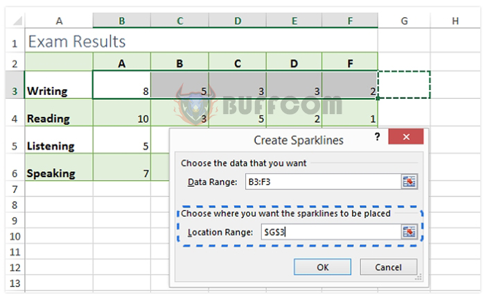
Step 1: Select the cells that are the data source for your mini-chart.
Step 2: Go to the Sparklines group on the INSERT tab and choose the desired type.
The Create Sparklines dialog box will appear on the screen. You will see the selected data range automatically displayed in the Data Range field.

Instructions for inserting Sparklines in Excel
Step 3: Select the cell where you want to place the Sparklines. You can simply click on the necessary cell or use the Select Range button to specify the location for your mini-chart. The cell reference will appear in the Location Range field.
Instructions for inserting Sparklines in Excel
Step 4: Click OK.
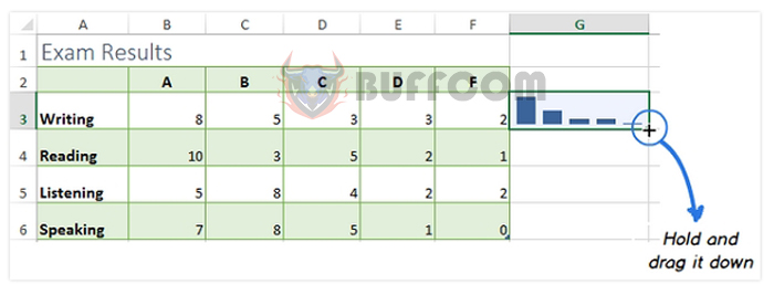
You will see the first Sparklines in the cell right next to your data source. If you want to apply it to all other data rows, you can easily do so by holding and dragging the mouse.
Instructions for inserting Sparklines in Excel
When you release the mouse button, the Sparklines will be inserted into adjacent cells.
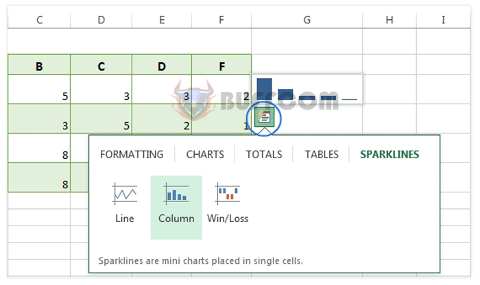
If you are using Excel 2013, you can use the Quick Analysis tool to quickly add Sparklines to your data. All you have to do is select the cells in the worksheet and click the Quick Analysis icon in the lower right corner of the selection area.
Instructions for inserting Sparklines in Excel
Then, switch to the SPARKLINES tab and choose the type. Note that if you use the Quick Analysis tool to insert Sparklines in Excel 2013, you can preview how your data will look with each type. Simply hover the cursor over the corresponding icon.


