Instructions on using shortcut keys to Group data in Excel quickly
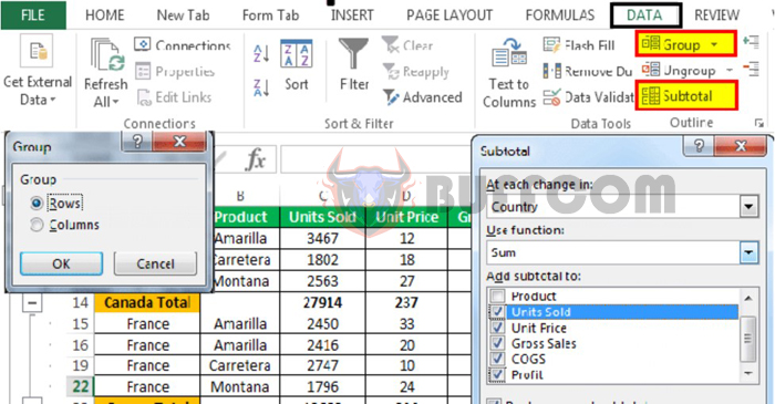
Using shortcut keys for Group in Excel is a quick way to hide/show or group rows/columns in an Excel spreadsheet. By using this method, you can save time from using the mouse and reduce errors from accidentally clicking on the wrong command button. Buffcom.net will guide you through using the Group shortcut keys in Excel easily and quickly.
1 What is Group in Excel?
To serve the purpose of data analysis and statistical work, Excel provides users with the Group function. Group in Excel allows you to easily group multiple columns or rows into one group, and you only need to perform a few steps to quickly hide and unhide data columns or rows in Excel.
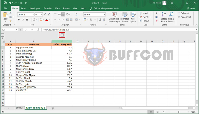
Looking at the illustration below, you can see that columns C, D, and E have been hidden.
Instructions on using shortcut keys to Group data in Excel quickly
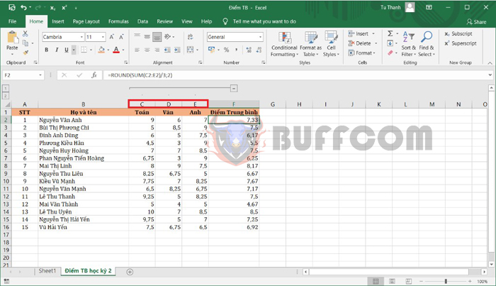
To display the hidden columns, you just need to click the plus sign on the worksheet. Immediately, the hidden 03 columns will be displayed.
Instructions on using shortcut keys to Group data in Excel quickly
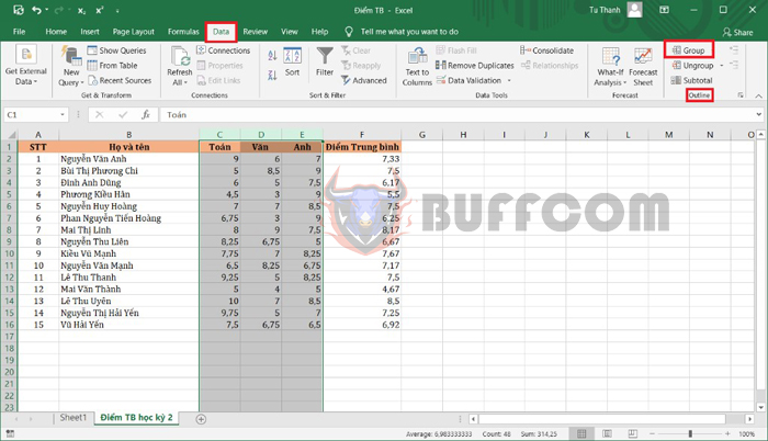
To create a Group in Excel, you usually need to select the columns or rows you want to group together. Then, on the toolbar, you go to the Data tab. Next, in the Outline group, you click on Group.
Instructions on using shortcut keys to Group data in Excel quickly
2 Shortcut Key for Group in Excel
To support users to the maximum extent, Excel has provided a shortcut key combination for Group in Excel. You can easily perform it without using the mouse or opening the Data tab.
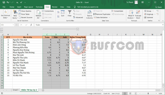
Step 1: You select the columns or rows that you want to create a Group.
Step 2: You use the Shift Alt → key combination to create a Group.
Then, the selected columns or rows will form a Group, as shown in the illustration below.
Instructions on using shortcut keys to Group data in Excel quickly
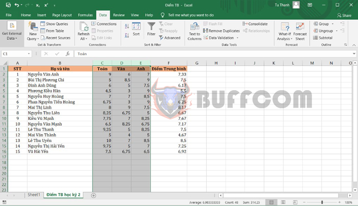
After that, you can easily click the minus sign to hide the columns in the Group. In addition, you can also create one or more Groups on the same worksheet, and easily delete a Group by using the Shift Alt ← key combination.
Instructions on using shortcut keys to Group data in Excel quickly
Thus, the article above from Buffcom.net has guided you on how to create and use the shortcut key for Group in Excel. Hopefully, this article will be useful for you in your work. Wish you success!


