3 Easy Ways to Get Month Names from Dates in Excel

3 Easy Ways to Get Month Names from Dates in Excel. During the process of handling time columns, you may want to extract the month or display the month name from the date. Below, I will show you 3 easy ways to get month names from dates in Excel. Let’s refer to the methods below!
3 Easy Ways to Get Month Names from Dates in Excel
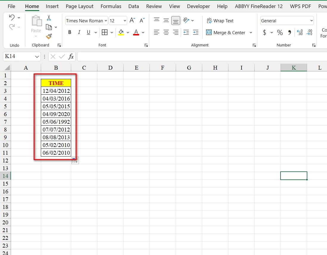
Example: Given the following data:
To get the month name based on the above data, you have 3 ways as follows:
Method 1: Get Month Name from Custom Number Format
3 Easy Ways to Get Month Names from Dates in Excel
3 Easy Ways to Get Month Names from Dates in Excel
Steps to perform:
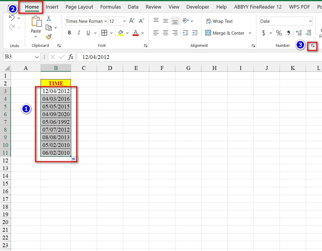
Step 1: Highlight the data range containing the time you want to display the month name.
Step 2: On the Home tab, click on the arrow on the right side of the Number group.
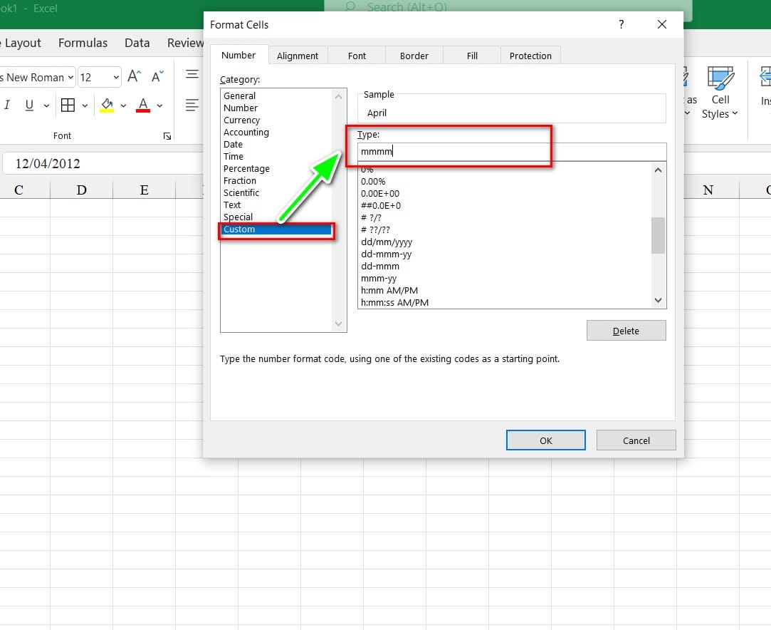
Step 3: The Format Cells dialog box appears. Select Custom and type “mmmm” in the Type box.
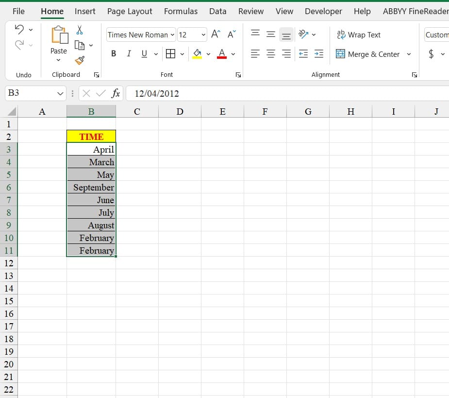
Step 4: Click OK to display the result.
3 Easy Ways to Get Month Names from Dates in Excel
Method 2: Get Month Name from Text Function
3 Easy Ways to Get Month Names from Dates in Excel
3 Easy Ways to Get Month Names from Dates in Excel
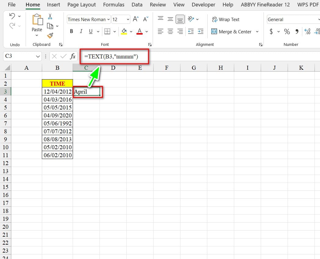
First, you select the cell to display the month name. Next, you enter the following formula: =TEXT(B3,”mmmm”)
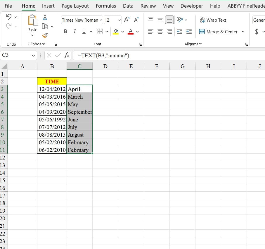
Finally, to display the cells below, you also highlight from the first cell to the last row and press Ctrl + D.
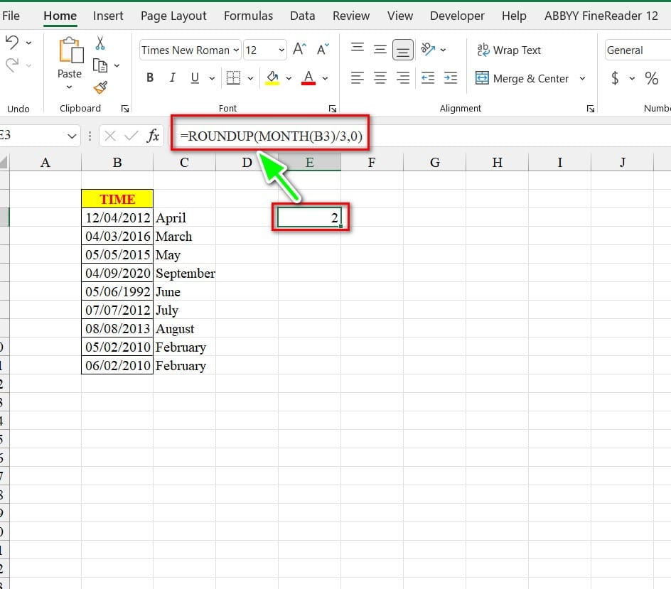
In addition, to calculate the quarter based on the month, use the formula: =ROUNDUP(MONTH(B3)/3,0).
3 Easy Ways to Get Month Names from Dates in Excel
Method 3: Get Month Name Using Power Query
Steps to perform:
Step 1: Select any cell in the data table, then go to the Insert tab, select Table and press OK to create a data table.
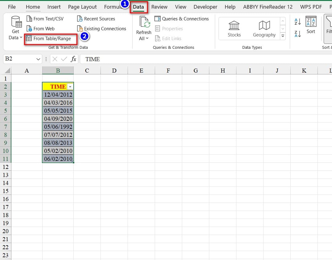
Step 2: In the data, go to the Data tab, select From Table/Range.
3 Easy Ways to Get Month Names from Dates in Excel
Step 3: The Power Query interface appears.
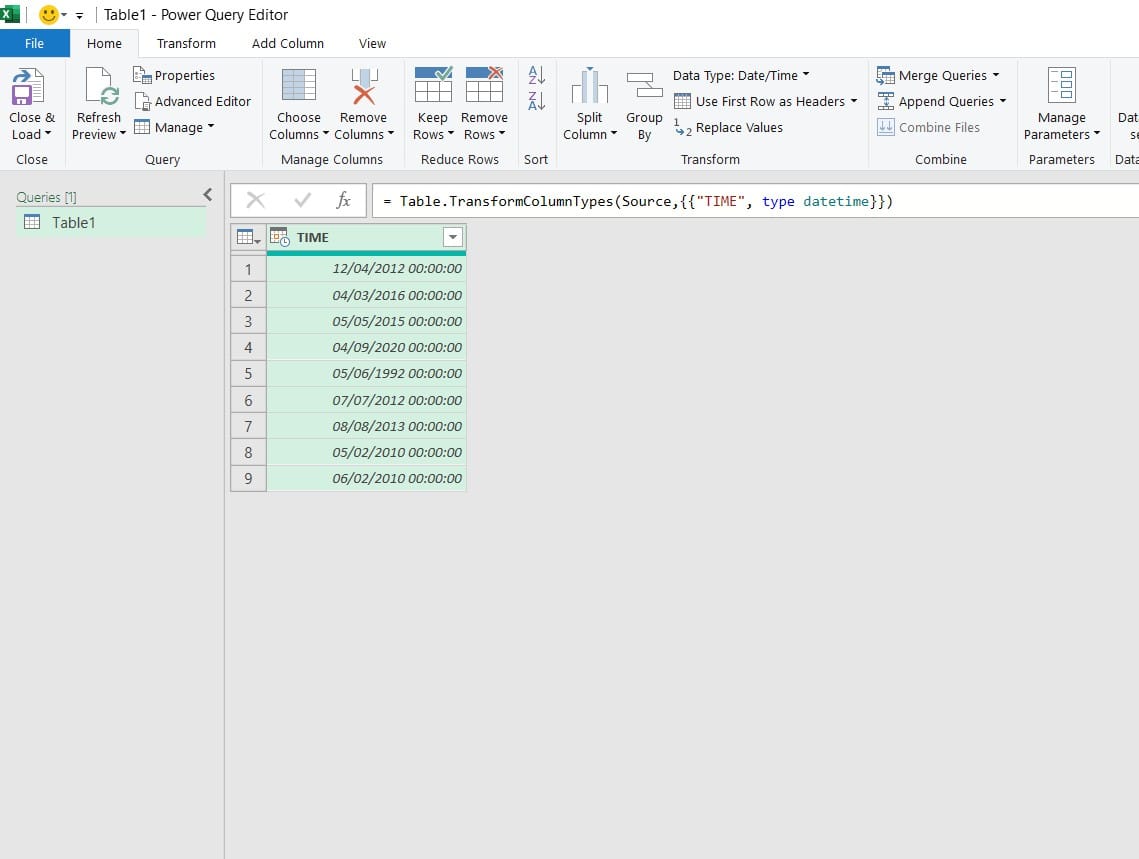
3 Easy Ways to Get Month Names from Dates in Excel
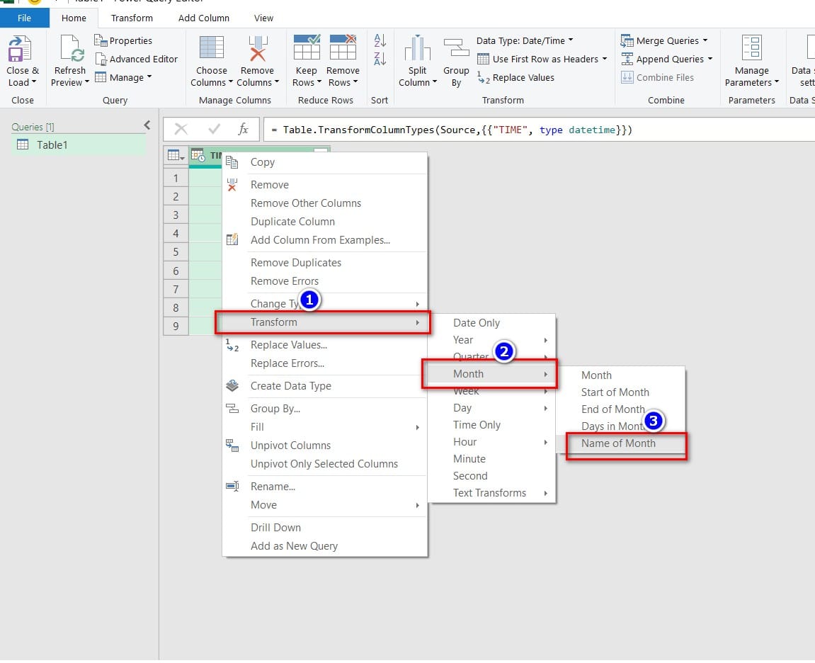
Step 4: Select the column header and right-click, select Transform, then select Month and Name of Month.
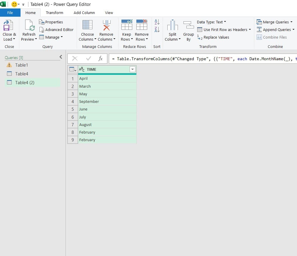
Step 5: The result is displayed.
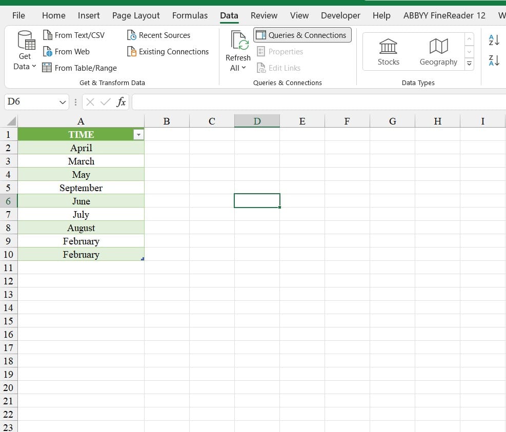
Step 6: To exit the Power Query interface, go to the Home tab and select Close & Load.
So, I have instructed you on 3 ways to display month names from dates in Excel. Good luck and if you find this helpful, don’t forget to rate the article below!


