Change the color in Google Sheets with just 2 clicks

Have you ever wanted to quickly alternate row colors in Google Sheets with just 2 clicks? Buffcom.net will show you how to do it using the built-in feature. This is a new feature recently added by Google Sheets to help users perform tasks more quickly.

Previously, you had to use conditional formatting to achieve this, but now you can do it with just 2 clicks. Additionally, this article also explains the conditional method for those who need to alternate 3 or 4 rows.

How to quickly alternate row colors in Google Sheets:

Assuming you already have a data table like the one below and you want to highlight/alternate row colors:

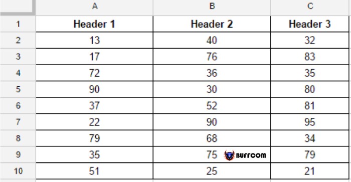Below are the steps:

Step 1. Select all cells in the data table (including the header).

Step 2. Go to the “Format” tab.

Step 3. Select “Alternating colors”.

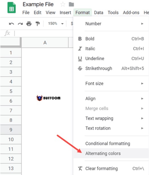Step 4. In the Alternating colors panel on the right, follow these instructions:

In the Styles option, make sure you have ticked the Header box. If your data table does not have a header, untick this box.

Choose one of the available templates, or you can also customize the colors for Header, Color 1, and Color 2 as desired.

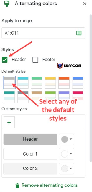Completing these steps will alternate the row colors in Google Sheets as shown below:

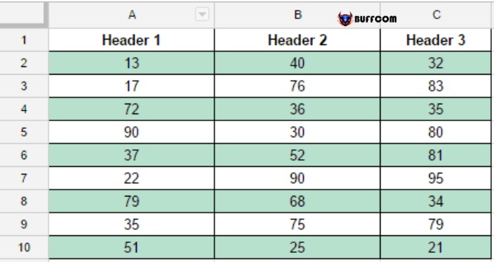To remove the alternating color, select any cell in the data table, go to the Format tab, and select Alternating colors. A control panel will open, where you can choose “Remove alternating color”.

Some things to keep in mind when using the Alternating colors feature in Google Sheets:

If you have already colored the data cells, using the Alternating colors feature will override the existing colors. When you remove the new color, the old color will remain.

If you want to change the color of a specific header or data cell, you can manually change it. This will override the existing color.

If you expand the data table and insert additional rows, Google Sheets will automatically highlight every other row with the selected color. However, when you delete a data row, the color will still remain and you have to manually delete it.

How to alternate color 3 or 4 rows in Google Sheets

To alternate color rows, the above method is the best and fastest. But if you don’t want to alternate every other row and instead want to alternate 3 or 4 rows at a time, what do you do?

For this case, you need to use the Conditional Formatting feature along with a simple formula.

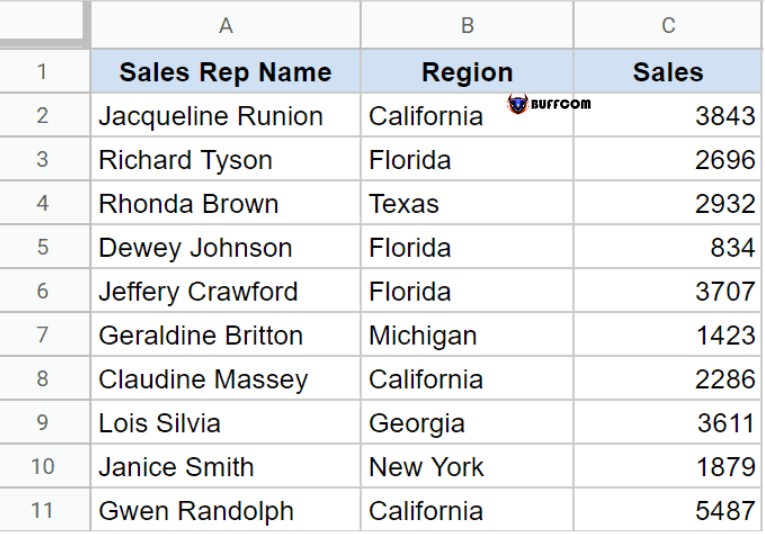
Assume you have a data table like the one below and you want to alternate color every 3 rows in this table:

Here are the steps:

Step 1. Select the data table that you want to alternate color every 3 rows (excluding the header).

Step 2. Select the Format tab.

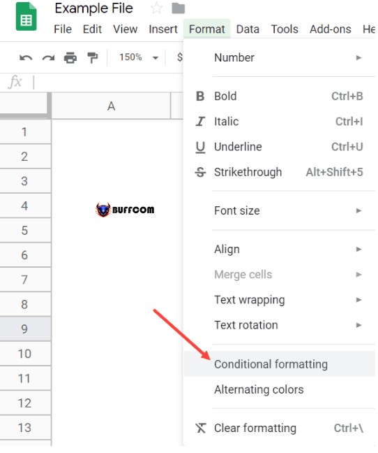
Step 3. Select the Conditional formatting option. This action will open the Custom Formatting panel on the right.

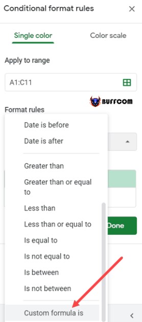
Step 4. In the Format rules menu, scroll down and select “Custom formula is”.

Step 5. In the “Value or Formula” box below, enter the following formula: =MOD(ROW(),3)-1=0.

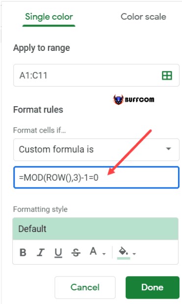Step 6. Select the formatting type. You can alternate color every 3 rows or bold, italicize, etc.

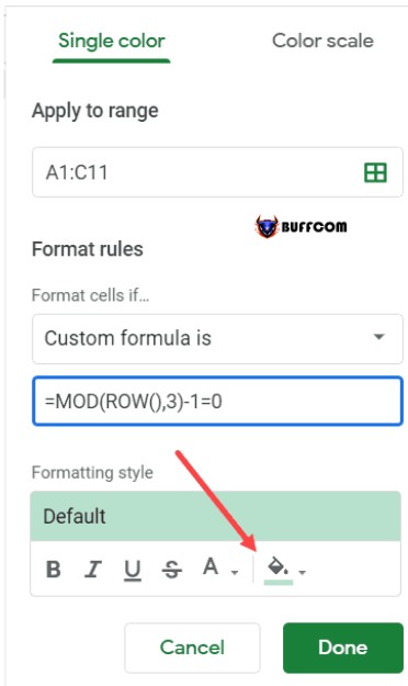Step 7. Select Done.

Performing the above steps will apply the selected format/color to alternate every 3 rows in Google Sheets.

That’s the guide on how to alternate row color in Google Sheets in a snap.

Hopefully, through this article, you will know how to alternate row color in Google Sheets using the Alternating colors feature. If you have any questions or feedback, please leave a comment for Buffcom.net. Wish you success.